Download
1 / 22
220 likes | 316 Views
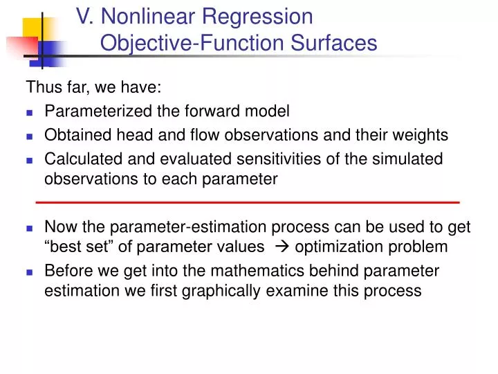
V. Nonlinear Regression Objective-Function Surfaces. Thus far, we have: Parameterized the forward model Obtained head and flow observations and their weights Calculated and evaluated sensitivities of the simulated observations to each parameter

E N D
V. Nonlinear Regression Objective-Function Surfaces Thus far, we have: • Parameterized the forward model • Obtained head and flow observations and their weights • Calculated and evaluated sensitivities of the simulated observations to each parameter • Now the parameter-estimation process can be used to get “best set” of parameter values optimization problem • Before we get into the mathematics behind parameter estimation we first graphically examine this process
V. Nonlinear Regression Objective-Function Surfaces Sum of squared weighted residuals objective function: HEADS FLOWS PRIOR Goal of nonlinear regression is to find the set of model parameters b that minimizes S(b)
Objective-Function Surfaces - continued • Weighted squared errors are dimensionless, so quantities with different units can be summed in the objective function. • Increasing the weight on an observation increases the contribution of that observation to S(b) .
Objective-Function Surfaces - continued • Objective function has as many dimensions as there are model parameters. For a 2-parameter problem, the objective function can be calculated for many pairs of parameter values, and the resulting objective-function surface can be contoured
Steady-State Problem as a Two-Parameter Problem • Original six-parameter model is re-posed so that the six defined parameters are combined to form two parameters: KMult and RchMult. [Problem with K_RB when using MODFLOW-2000. Omission from KMult not problematic because K_RB is insensitive]. • When KMult = 1.0: • Like when HK_1, HK_2, VK_CB, and K_RB equal their starting values in the six-parameter model. • When Rch_Mult = 1.0: • Like when RCH_1 and RCH_2 equal their starting values in the six-parameter model.
Steady-State Problem as a Two-Parameter Problem • With the problem posed in terms of KMult and RchMult: • Use UCODE_2005 in Evaluate Objective Function mode to calculate S(b) using many sets of values for KMult and RchMult • Values of KMult and RchMult range from 0.1 to 10 • Use many values for each within this range. If 100, would have 100x100=10,000 sets of parameter values • Plot values of S(b) for each set of parameter values • Contour the resulting objective-function surface • Examine how the objective-function surface changes given different observation types and weights.
Steady-State Problem as a Two-Parameter Problem Objective function surfaces (Book, Fig. 5-4, p. 82)(contours of objective function calculated for combinations of 2 parameters) With flow weighted using a coefficient of variation of 1% With flow weighted using a coefficient of variation of 10% Heads only
Why aren’t the objective functions symmetric about he minimum? (the trough when correlated) Parameter Nonlinearity of Darcy’s Law(Hill and Tiedeman, 2007, p. 12-13) • Darcy’s Law Q = -KA • h = h0 - (Q/KA) X = - Linear = - X Nonlinear in K = - X Nonlinear in K Nonlinearity makes it much harder to estimate parameter values.
DO EXERCISE 5.1a: Assess relation of objective-function surfaces to parameter correlation coefficients.
Exercise 5.1a - questions • Use Darcy’s Law to explain why all the parameters are completely correlated when only hydraulic-head observations are used. • Why does adding a single flow measurement make such a difference in the objective-function surface? • Given that addition of one observation prevents the parameters from being completely correlated, what effect do you expect any error in the flow measurement to have on the regression results?
Why aren’t the objective functions symmetric about he minimum? (the trough when correlated) Parameter Nonlinearity of Darcy’s Law(Hill and Tiedeman, 2007, p. 12-13) • Darcy’s Law Q = -KA • h = h0 - (Q/KA) X = - Linear = - X Nonlinear in K = - X Nonlinear in K Nonlinearity makes it much harder to estimate parameter values.
Introduction to the Performance of the Gauss-Newton Method: Effect of MAX-CHANGE • Goal of the modified Gauss-Newton (MGN) method: find the minimum value of the objective function. • MGN iterates. Each iteration moves toward the minimum of an approximate objective function. Approximation: linearize the model about the current set of parameter values. • If the approximate and true objective functions are very different, the minimum of the approximate objective-function may be far from the true minimum. • Often advantageous to restrict the method: for any one iteration the parameter values are not allowed to change too much. Use damping. • MAX-CHANGE: User-specified value partly controls the damping. MAX-CHANGE = the maximum fractional change allowed in one regression iteration. If MAX-CHANGE=2 and the parameter value=1.1, the new value is allowed to be between 1.1±(2x1.1), or between -1.1 and 3.3.
DO EXERCISE 5.1b: Examine the performance of the modified Gauss-Newton method for the two-parameter lumped problem.
Exercise 5.1b – questions in first bullet • Do the regression runs converge to optimal parameter values? • How do the estimated parameter values compare among the different regression runs? • Explain the difference in the progression of parameter values during these regression runs.
Exercise: Plot regression results on objective function surface for model calibrated with ONLY HEAD DATA • 4 regression runs with different starting values or different maximum step sizes: • Run 1: Start near trough • Run 2: Start far away, let regression take big steps • Runs 3 & 4: Start far away, force small steps • The regression converged in 3 of the runs! • Are those parameter estimates unique?
Exercise: Plot regression results on objective function surface for model calibrated with HEAD AND FLOW DATA • Same starting values and maximum step sizes as in previous exercise. • The regression again converged in 3 of the runs. • Now do we have a calibrated model with unique parameter estimates?
~Var(b2) ~Var(b1) Effects of Correlation and Insensitivity b2 Linear objective function: No correlation, b1 less sensitive minimum b1
Effects of Correlation and Insensitivity b2 Linear objective function Strong, negative correlation minimum b1
Effects of Correlation and Insensitivity objective function value Minimum is not well defined Parameter values along section
~Var(b2) ~Var(b1) Effects of Correlation and Insensitivity b2 Linear objective function Strong, negative correlation minimum b1
Effects of Correlation and Insensitivity • Insensitivity • Stretches the contours in the direction of the insensitive parameter. • very insensitive = very uncertain • Correlations • Rotate the contours away from the parameter axis • Uncertainty from one parameter can be passed into another parameter! • Create parameter combinations that give equivalent results • Increases the non-uniqueness