Download
1 / 45
470 likes | 503 Views
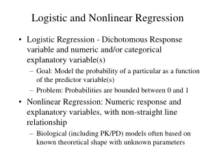
Learn about popular nonlinear regression models like Exponential, Power, and Saturation Growth for given data sets in this educational guide. Discover how to find constants using numerical methods and apply models to real-world examples. Explore Polynomial models and linearization techniques for nonlinear data. Get ready to enhance your skills in nonlinear regression analysis for STEM applications.

E N D
Nonlinear Regression Chemical Engineering Majors Authors: Autar Kaw, Luke Snyder http://numericalmethods.eng.usf.edu Transforming Numerical Methods Education for STEM Undergraduates http://numericalmethods.eng.usf.edu
Nonlinear Regression Some popular nonlinear regression models: 1. Exponential model: 2. Power model: 3. Saturation growth model: 4. Polynomial model:
Nonlinear Regression Given n data points best fit to the data, where is a nonlinear function of . Figure. Nonlinear regression model for discrete y vs. x data
Exponential Model Given best fit to the data. Figure. Exponential model of nonlinear regression for y vs. x data
Finding constants of Exponential Model The sum of the square of the residuals is defined as Differentiate with respect to a and b
Finding constants of Exponential Model Rewriting the equations, we obtain
Finding constants of Exponential Model Solving the first equation for yields Substituting back into the previous equation Nonlinear equation in terms of The constant can be found through numerical methods such as the bisection method or secant method.
Example 1-Exponential Model Many patients get concerned when a test involves injection of a radioactive material. For example for scanning a gallbladder, a few drops of Technetium-99m isotope is used. Half of the techritium-99m would be gone in about 6 hours. It, however, takes about 24 hours for the radiation levels to reach what we are exposed to in day-to-day activities. Below is given the relative intensity of radiation as a function of time. Table. Relative intensity of radiation as a function of time.
Example 1-Exponential Model cont. The relative intensity is related to time by the equation Find: a) The value of the regression constants and b) The half-life of Technium-99m c) Radiation intensity after 24 hours
Constants of the Model The value of λis found by solving the nonlinear equation
Setting up the Equation in MATLAB t=[0 1 3 5 7 9] gamma=[1 0.891 0.708 0.562 0.447 0.355] syms lamda sum1=sum(gamma.*t.*exp(lamda*t)); sum2=sum(gamma.*exp(lamda*t)); sum3=sum(exp(2*lamda*t)); sum4=sum(t.*exp(2*lamda*t)); f=sum1-sum2/sum3*sum4;
Calculating the Other Constant The value of A can now be calculated The exponential regression model then is
Relative Intensity After 24 hrs The relative intensity of radiation after 24 hours This result implies that only radioactive intensity is left after 24 hours.
Homework • What is the half-life of technetium 99m isotope? • Compare the constants of this regression model with the one where the data is transformed. • Write a program in the language of your choice to find the constants of the model.
THE END http://numericalmethods.eng.usf.edu
Polynomial Model Given best fit to a given data set. Figure. Polynomial model for nonlinear regression of y vs. x data
Polynomial Model cont. The residual at each data point is given by The sum of the square of the residuals then is
Polynomial Model cont. To find the constants of the polynomial model, we set the derivatives with respect to where equal to zero.
Polynomial Model cont. These equations in matrix form are given by The above equations are then solved for
Example 2-Polynomial Model Below is given the FT-IR (Fourier Transform Infra Red) data of a 1:1 (by weight) mixture of ethylene carbonate (EC) and dimethyl carbonate (DMC). Absorbance P is given as a function of wavenumber m. Table. Absorbance vs Wavenumber data Figure. Absorbance vs. Wavenumber data http://numericalmethods.eng.usf.edu
Example 2-Polynomial Model cont. Regress the data to a second order polynomial where and find the absorbance at The coefficients are found as follows http://numericalmethods.eng.usf.edu
Example 2-Polynomial Model cont. The necessary summations are as follows Table. Necessary summations for calculation of polynomial model constants http://numericalmethods.eng.usf.edu
Example 2-Polynomial Model cont. Necessary summations continued: Table. Necessary summations for calculation of polynomial model constants. http://numericalmethods.eng.usf.edu
Example 2-Polynomial Model cont. Using these summations we have Solving this system of equations we find The regression model is then http://numericalmethods.eng.usf.edu
Example 2-Polynomial Model cont. With the model is given by Figure. Polynomial model of Absorbance vs. Wavenumber. http://numericalmethods.eng.usf.edu
Example 2-Polynomial Model cont. To find where we have http://numericalmethods.eng.usf.edu
Linearization of Data To find the constants of many nonlinear models, it results in solving simultaneous nonlinear equations. For mathematical convenience, some of the data for such models can be linearized. For example, the data for an exponential model can be linearized. As shown in the previous example, many chemical and physical processes are governed by the equation, Taking the natural log of both sides yields, Let and We now have a linear regression model where (implying) with
Linearization of data cont. Using linear model regression methods, Once are found, the original constants of the model are found as
Example 3-Linearization of data Many patients get concerned when a test involves injection of a radioactive material. For example for scanning a gallbladder, a few drops of Technetium-99m isotope is used. Half of the technetium-99m would be gone in about 6 hours. It, however, takes about 24 hours for the radiation levels to reach what we are exposed to in day-to-day activities. Below is given the relative intensity of radiation as a function of time. Table. Relative intensity of radiation as a function of time Figure. Data points of relative radiation intensity vs. time
Example 3-Linearization of data cont. Find: a) The value of the regression constants and b) The half-life of Technium-99m c) Radiation intensity after 24 hours The relative intensity is related to time by the equation
Example 3-Linearization of data cont. Exponential model given as, Assuming , and we obtain This is a linear relationship between and
Example 3-Linearization of data cont. Using this linear relationship, we can calculate where and
Example 3-Linearization of Data cont. Summations for data linearization are as follows With Table. Summation data for linearization of data model
Example 3-Linearization of Data cont. Calculating Since also
Example 3-Linearization of Data cont. Resulting model is Figure. Relative intensity of radiation as a function of temperature using linearization of data model.
Example 3-Linearization of Data cont. The regression formula is then b) Half life of Technetium 99 is when
Example 3-Linearization of Data cont. c) The relative intensity of radiation after 24 hours is then This implies that only of the radioactive material is left after 24 hours.
Comparison Comparison of exponential model with and without data linearization: Table. Comparison for exponential model with and without data linearization. The values are very similar so data linearization was suitable to find the constants of the nonlinear exponential model in this case.
Additional Resources For all resources on this topic such as digital audiovisual lectures, primers, textbook chapters, multiple-choice tests, worksheets in MATLAB, MATHEMATICA, MathCad and MAPLE, blogs, related physical problems, please visit http://numericalmethods.eng.usf.edu/topics/nonlinear_regression.html
THE END http://numericalmethods.eng.usf.edu