Download
1 / 44
440 likes | 643 Views
Shortest Paths (Review). Single Source Shortest Path. Dijkstra’s Algorithm Label Path length to each vertex as (or 0 for the start vertex) Loop while there is a vertex Remove up the vertex with minimum path length Check and if required update the path length of its adjacent neighbors

E N D
Single Source Shortest Path • Dijkstra’s Algorithm • Label Path length to each vertex as (or 0 for the start vertex) • Loop while there is a vertex • Remove up the vertex with minimum path length • Check and if required update the path length of its adjacent neighbors • end loop Update rule: Let ‘a’ be the vertex removed and ‘b’ be its adjacent vertex Let ‘e’ be the edge connecting a to b. if (a.pathLength + e.weight < b.pathLength) b.pathLengtha.PathLength + e.weight b.parent a 6 6 D D 5 C C 10 1 1 6 6 8 8 E E 6 5 5 6 6 7 7 2 2 B B A A 2
Single Source Shortest Path • DAG based Algorithm May have negative weight • Label Path length to each vertex as (or 0 for the start vertex) • Compute Topological Ordering • loop for i 1 to n-1 • Check and if required update the path length of adjacent neighbors of vi • end loop Path Length from A To i=1 i=2 i=3 i=4 -2 D C 3 B -5 8 E 5 C 6 9 D 2 B A E
All-Pairs Shortest Paths Uses only vertices numbered 1,…,k (compute weight of this edge) i j Uses only vertices numbered 1,…,k-1 k Uses only vertices numbered 1,…,k-1
All-Pairs Shortest Paths Dynamic Programming approach • Initialize a nn table with 0 or or edge length. • Check and Update the table bottom up in nested loops for k, for i, for j j i -2 D C 3 -5 8 E 5 6 9 2 B A
Minimum Spanning Trees 2704 BOS 867 849 PVD ORD 187 740 144 JFK 1846 621 1258 184 802 SFO BWI 1391 1464 337 1090 DFW 946 LAX 1235 1121 MCO 2342
Spanning subgraph Subgraph of a graph G containing all the vertices of G Spanning tree Spanning subgraph that is itself a (free) tree Minimum spanning tree (MST) Spanning tree of a weighted graph with minimum total edge weight Applications Communications networks Transportation networks Minimum Spanning Tree ORD 10 1 PIT DEN 6 7 9 3 DCA STL 4 5 8 2 DFW ATL
Cycle Property 8 f 4 C Cycle Property: • Let T be a minimum spanning tree of a weighted graph G • Let e be an edge of G that is not in T • Let C let be the cycle formed by e with T • For every edge f of C,weight(f) weight(e) Proof: • By contradiction • If weight(f)> weight(e) we can get a spanning tree of smaller weight by replacing e with f 9 6 2 3 e 7 8 7 Replacing f with e yieldsa better spanning tree 8 f 4 C 9 6 2 3 e 7 8 7
Partition Property U V 7 f 4 9 Partition Property: • Consider a partition of the vertices of G into subsets U and V • Let e be an edge of minimum weight across the partition • There is a minimum spanning tree of G containing edge e Proof: • Let T be an MST of G • If T does not contain e, consider the cycle C formed by e with T and let f be an edge of C across the partition • By the cycle property,weight(f) weight(e) • Thus, weight(f)= weight(e) • We obtain another MST by replacing f with e 5 2 8 3 8 e 7 Replacing f with e yieldsanother MST U V 7 f 4 9 5 2 8 3 8 e 7
Minimum Spanning Tree • Prim’s Algorithm (Prim-Jarnik Algorithm) • Label cost of each vertex as (or 0 for the start vertex) • Loop while there is a vertex • Remove a vertex that will extend the tree with minimum additional cost • Check and if required update the path length of its adjacent neighbors (Update rule different from Dijkstra’s algorithm) • end loop Update rule: Let ‘a’ be the vertex removed and ‘b’ be its adjacent vertex Let ‘e’ be the edge connecting a to b. if (e.weight < b.cost) b.coste.weight b.parent a 6 D C 1 6 8 E 2 6 7 2 B A
MST: Prim-Jarnik’s Algorithm 6 D C 1 6 8 E 6 2 7 2 B A 0
MST: Prim-Jarnik’s Algorithm 6 D C 1 2,A 6 8 E 6 2 7,A 7 2 B A 2,A 0
MST: Prim-Jarnik’s Algorithm 6 D C 1 2,A 6 8 E 6 2 7,A 7 2 B A 2,A 0
MST: Prim-Jarnik’s Algorithm 6 D 8,B C 1 2,A 6 8 E 6 2 6,B 7 2 B A 2,A 0
MST: Prim-Jarnik’s Algorithm 6 D 8,B C 1 2,A 6 8 E 6 2 6,B 7 2 B A 2,A 0
MST: Prim-Jarnik’s Algorithm 6 D 6,D C 1 2,A 6 8 E 6 2 1,D 7 2 B A 2,A 0
MST: Prim-Jarnik’s Algorithm 6 D 6,D C 1 2,A 6 8 E 6 2 1,D 7 2 B A 2,A 0
MST: Prim-Jarnik’s Algorithm 6 D 6,D C 1 2,A 6 8 E 6 2 1,D 7 2 B A 2,A 0
MST: Prim-Jarnik’s Algorithm 6 D 6,D C 1 2,A 6 8 E 6 2 1,D 7 2 B A 2,A 0
Prim-Jarnik Algorithm AlgorithmMST (G) Q new priority queue Let s be any vertex for allv G.vertices() if v = s v.cost 0 else v.cost v. parent null Q.enQueue(v.cost, v) whileQ.isEmpty() • v Q .removeMin() • v.pathKnown true • for alle G.incidentEdges(v) w opposite(v,e) if w.pathKnown if weight(e) < w.cost w.cost weight(e) w. parent v update key of win Q O(n) O(n log n) O((n+m) log n)
7 7 D 2 B 4 9 5 5 F 2 C 8 3 8 E A 7 7 0 7 7 7 D 2 7 D 2 B 4 B 4 9 5 4 9 5 5 F 2 5 F 2 C 8 C 8 3 3 8 8 E E A 7 7 A 7 0 7 0 Example 7 D 2 B 4 9 8 5 F 2 C 8 3 8 E A 7 7 0
7 7 D 2 B 4 4 9 5 5 F 2 C 8 3 8 E A 3 7 0 Example (contd.) 7 7 D 2 B 4 4 9 5 5 F 2 C 8 3 8 E A 3 7 0
Minimum Spanning Tree • Kruskal’s Algorithm • Create a forest of n trees • Loop while (there is > 1 tree in the forest) • Remove an edge with minimum weight • Accept the edge only if it connects 2 trees from the forest in to one. • end loop 6 D C 1 6 8 E 2 6 7 E D C B A 2 B A
MST: Kruskal’s Algorithm 6 D C 1 6 8 E 2 6 7 2 B A E D C B A
MST: Kruskal’s Algorithm 6 D C 1 6 8 E 2 6 7 2 B A E D C B A
MST: Kruskal’s Algorithm 6 D C 1 6 8 E 2 6 7 2 B A E D C B A
MST: Kruskal’s Algorithm 6 D C 1 6 8 E 2 6 7 2 B A E D C B A
Kruskal’s Algorithm AlgorithmKruskalMST(G) letQbe a priority queue. Insert all edges into Q using their weights as the key Create a forest of n trees where each vertex is a tree numberOfTrees n whilenumberOfTrees > 1do edge eQ.removeMin() Let u, v be the endpoints of e ifTree(v) Tree(u)then Combine Tree(v)and Tree(u) using edge e decrement numberOfTrees return T O(m log m) O(m log m)
2704 BOS 867 849 PVD ORD 187 740 144 JFK 1846 621 1258 184 802 SFO BWI 1391 1464 337 1090 DFW 946 LAX 1235 1121 MIA 2342 Kruskal Example
2704 BOS 867 849 PVD ORD 187 740 144 JFK 1846 621 1258 184 802 SFO BWI 1391 1464 337 1090 DFW 946 LAX 1235 1121 MIA 2342 Example
Minimum Spanning Tree • Baruvka’s Algorithm • Create a forest of n trees • Loop while (there is > 1 tree in the forest) • For each tree Ti in the forest • Find the smallest edge e = (u,v), in the edge list with u in Ti and v in TjTi • connects 2 trees from the forest in to one. • end loop 6 D C 1 6 8 E 5 6 7 E D C B A 2 B A
Baruvka’s Algorithm • Like Kruskal’s Algorithm, Baruvka’s algorithm grows many “clouds” at once. • Each iteration of the while-loop halves the number of connected compontents in T. • The running time is O(m log n). AlgorithmBaruvkaMST(G) T V{just the vertices of G} whileT has fewer than n-1 edges do for each connected component C in Tdo Let edge e be the smallest-weight edge from C to another component in T. ife is not already in Tthen Add edge e to T return T