Download
1 / 43
430 likes | 510 Views
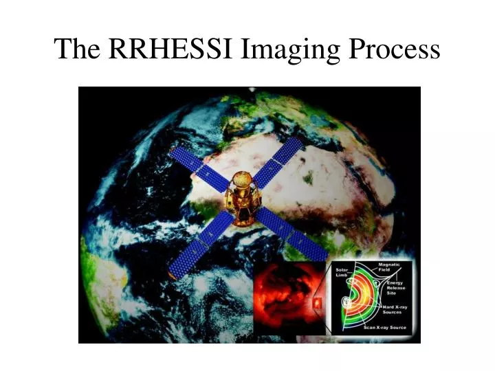
The RRHESSI Imaging Process. How RHESSI Images. Making RHESSI images of solar flares is a 2-step process.

E N D
How RHESSI Images Making RHESSI images of solar flares is a 2-step process. Step1: Varying fractions of the X-rays and gamma-rays emitted by a solar flare are detected by the germanium detectors on the RHESSI spacecraft and the measurements are radioed to a ground station. Step 2: Information about each detected photon and the exact direction that the instrument was pointing is used in computers on the ground to make the images.
How RHESSI Images Step 1 • The grid pairs modulate transmission of flare X-ray and gamma-ray photons to the detectors. • Fraction of the photons that make it through both grids to the detector varies with time • This fraction varies between zero and about 50% as the spacecraft rotates.
How RHESSI Images • First, consider a steady point source of X-rays on the Sun • X-ray photons from the source travel in all directions. We are only concerned with those that reach RHESSI.
The Sun is so far away (93 million miles or 1.5 x 10¹¹ m) compared to the diameter of the RHESSI grid tray (~1 m). • The largest possible angle between the paths of any 2 photons detected by RHESSI is 1 m/1.5 x 1011 m x 360/2 pi degrees = 1.2 x 10⁻⁶ arcseconds • This is so small compared to RHESSI’s finest resolution of 2 arcseconds. • Thus, all photons that reach RHESSI can be considered to be traveling on parallel paths
Timing Considerations • RHESSI is rotating at 15 rpm. • The time it takes a photon traveling at the speed of light (186,000 miles per second or 3 x 1010 cm s‑1) to move the 1.55 m between the front and rear grids is only (1.55 * 102)/(3 * 1010) s = 5.2 * 10-9 s. • At the 15 rpm rotation rate, even the grids near the edge of the trays move a very small distance in this time 2 x 50 x 5.2 x 10‑9/4 cm = 0.004 microns • This is small compared to the finest slit width of 20 microns. • Thus, we can ignore this small rotation that takes place as the photons pass from the front girds to the rear grids.
Components of Animations FrontGrid Rear Grid Detector This shows the color scheme in the following Flash animations.
Transmission Fraction • The area of each detector (yellow) seen through the front and rear grids tells you how many of the photons riding along with you in the virtually parallel beam from the common point source will be recorded by RHESSI at any given time. • The number of photons on the parallel beam that will be recorded by RHESSI changes between ~50% of the photons (when the slats of the front grid do not block any part of the rear slits) and no photons (when the slats of the front grid completely cover the slits of the rear grid). 50% transmission 0% transmission
View from a Point Source Located Exactly on the RHESSI Spin Axis • Imagine yourself riding along on one of the photons as you head towards RHESSI. • This animation shows what you would see assuming you were traveling exactly along the RHESSI spin axis. • The fraction of the detector area (shown in yellow) would stay constant as the spacecraft rotated. • The thermal insulation blankets and cryostat cover used to keep the instrument cool are transparent to all but the lowest energy X-rays.
Point Source Exactly on the Spin Axis • Since all detected photons from the point source can be considered as traveling on parallel paths, we can simplify the animation to show a single coarse collimator rotating about its center. • There is no change in the fraction of the detector area that is visible to the source as the spacecraft rotates. • The detector records a steady rate of photons equal to about half of the rate it would have seen if the grids were not there.
Point Source Exactly on the Spin Axis • In practice, the slats in the front grids are not exactly over the slats in the rear grids. • Thus, the fraction of the detector visible from the on-axis point source will be less than 50%. • The exact offset of the front and rear grids will be determined from the first flares detected.
Point Source below the Spin Axis • This is the view of both grid trays and all nine detectors from a point on the Sun below the RHESSI spin axis. • Note that the slits in the grids are too fine to be simulated in this animation and the modulation you see here is not real.
Point Source below the Spin Axis • As before, we can simulate what happens with a single coarse collimator rotating about its center. • Note that in this case, the front and rear grids no longer appear concentric when viewed from the source. • The area of the detector (yellow) visible through both grids changes with time as the spacecraft rotates. • Consequently, the detector counting rate also changes with time.
Point source below the spin axis • We can simplify the animation by considering the view if we rotate with the spacecraft. • The fraction of the detector area visible to the source changes in exactly the same way as in the previous animation. • We note that the visible area of the detector changes when the top grid moves up and down but not when it moves left to right.
Point source below the spin axis • In this animation, we show only the up and down motion (should be simple harmonic). of the front grid • The area of the detector visible at any time changes in exactly the same way as for the previous two animations. • This perspective allows us to see more clearly how the visible detector area changes with rotation.
Light Curve • Graph shows how the fraction of photons that make it through the two grids and reach the detector changes from zero to 50% as the spacecraft rotates. • The transmission fraction is the same as the fraction of the detector area that is visible from the source through the two grids as shown in the previous animations. • It takes 4 s to generate this light curve at 15 rpm.
Interpretation of Light Curves • Light curves provide information about the location, intensity, and extent of the source as follows: • The number of peaks gives the angular distance of the source from spin axis. • The rotation angle at time of slowest modulation gives the azimuth angle of source. • The mean count rate gives the intensity of the source. • The count rate in the valleys and the amplitude of the modulation gives an indication of the angular extent of the source compared to the resolution of the subcollimator.
Examples of Light Curves Produced by Different Sources Location of source & spin axis on Sun Count rate 0° 360° Rotation Angle P is the angular pitch of the subcollimator
How RHESSI Images Step 2 • Construct images from the telemetered data on each photon. • Simplest method is Back Projection.
Back Projection • Possible paths that a detected photon could have traveled. • Tracing these paths back to the Sun produces a map on the sky made up of many parallel lines showing where the photon could have originated. • The photon could not have originated from a point on the Sun between the lines because if it had, it would have been stopped by the slats in one of the grids and would not have reached the detector.
These six boxes show how a single point source can be located on the Sun using back- projection. The varying X-ray or gamma-ray counting rate measured by the detector behind the grids is transformed into an image of the flare. Back-Projection Animations
This box shows the area of the detector (yellow) seen by the source through the front grid (red) and the rear grid (blue). As the spacecraft rotates, the area of the detector visible to the source varies systematically between 0 and 50%. Visible Detector Area
This box shows how the detector counting rate changes with time. white = maximum counting rate black = minimum counting rate Detector Count Rate
This box shows the light curve of the detector counting rate. The counting rate is proportional to the area of the detector that is visible to the source through the grids. Count Rate Light Curve
This box contains a probability map of the Sun at one instant during the spacecraft rotation. White represents high probability, black is low probability that a detected photon at that time could have originated from that location on the Sun. The source is shown in the bottom left hand corner of the box. The spacecraft axis of rotation is shown by the cross in the center of the box. Back-projection Probability Map
These boxes show how the probability maps, weighted by the varying counting rate as the spacecraft rotates, are added together to produce the image of the source. The true source is seen in the bottom left corner. The “ghost” source in the upper right-hand corner appears because a source at that location would produce a similar light curve. Accumulated Probabilities
Single photon 10 deg rotation 90 deg rotation Multiple rotations Grids 3 – 8 Clean
Algorithms: Back Projection CONCEPT • Calculates a ‘probability map’ of photon’s origin on the Sun for each detected count. • Adds probability maps for all photons • Applies a flat-fielding correction to remove false source at spin axis. RESULT • Map represents a convolution of true map and point response function PROPERTIES • Real sources have significant circular sidelobes. • Can be directly interpreted only in simple situations • Relatively fast • Very robust • No a priori assumptions about source geometry
Modulation Properties (1) • Imaging is independent of background to first order since it is not modulated • Can ignore ‘background subtraction’ for imaging. • But background + all other sources contribute to noise. • An RMC does not modulate source components that are larger than its resolution Thus, using fine RMC’s does not help if source is extended. • Coarse collimators only give position and total strength of compact sources. Thus, including coarse collimators may not improve image quality.
Modulation Properties (2) • At least ½ rotation needed to produce modulation that is sensitive to source structure as viewed from all orientations. • Thus, best image quality if integration time is at least 2s (integer number of 4s intervals is better) • Distance of source from spin axis (and RMC resolution) determine modulation frequency. • Source structure determines amplitude and phase of modulation. • ~103 independent amplitudes and phases • Thus, only sources with simple spatial structure can be well-imaged.
“CLEANing” the Image • The back-projection image is known as a “dirty” image. It has many artifacts - mainly rings around each point source - that degrade the image. • The “dirty” image can be refined with a process called “CLEAN” • The known artifacts are subtracted out, one source at a time to leave an image that more closely represents the true source distribution.
The “Clean” Process • The pixel with the highest intensity in the “dirty map” created by back-projection is identified. • A point source with a fraction (called the “gain”) of the intensity in that pixelis assumed at that location. The default value of the gain is 10%. • The known distribution, including all the artifacts, for a point source with that intensity at that location is subtracted from the dirty map. • A gaussian source with a width equal to the resolution of the particular grids being used, and with the same intensity and location, is added to the CLEAN map. • Steps 1 – 4 are repeated until the remaining counts in the dirty map are all below some threshold level.
Other Image Reconstruction Algorithms • Other algorithms make assumptions about source geometry and use this information to improve map quality. • Clean • Assumes source is made up of a set of point sources. Usually works well. • Maximum Entropy Method (MEM) • Determines map consistent with least information content about source. • MEM-NJIT • PIXONS • Constructs the simplest source model that is consistent with the data. (Slow, but can give the best results) • Forward-Fitting • Assumes map is made up of a set of simple source components (Gaussians, etc) and determines the parameters of these components.
The Maximum Entropy Method (MEM) • MEM is a more sophisticated image reconstruction method. • The computer searches for a source distribution that is as smooth as possible while accurately reproducing the measured count-rate light curves from all of the selected detectors. • Entropy is a measure of the smoothness of the image. • Chi-squared is a measure of the accuracy of the fit to the light curves. • The final image has the highest possible entropy while still having an “acceptable” value of chi-squared. The default “acceptable” value is a reduced chi-squared of one.
Numerical example • Grid 1: 35 microns, 1.55m, 7cm diameter • Twist of 35microns/7cm smears source over 1 modulation cycle zero modulation. • Compare twist tolerance to angular resolution!
Exercise 1 • Consider RHESSI grid 1: • 34 micron pitch • 25 micron apertures • 1 mm thick • separated by 1.55m • Grids 9 cm in diameter • Detector 6 cm in diameter • What is the FWHM resolution of RMC1 (assume 1st harmonic only) ? • How much relative twist is required to totally destroy the modulation? • What would be the qualitative and quantitative effect of a relative twist of ½ of this amount ?
Exercise 2 Spin axis at [246,-73 ] Grid 8 slits were pointed at solar north at 18:58:08.5 UT and rotating at 15 rpm (clockwise looking at rear of collimator) What is the source location? Bonus questions: What is effect of a 1 arcminute error in the pointing? a 1 arcminute error in the aspect solution? a 1 acminute error in the roll aspect? Do a back projection image grid 8, 28-aug-2002 185750-185850 and compare to your estimate. Alternatively, use his_vis_fwdfit on the visibilities.