Download
1 / 74
740 likes | 771 Views
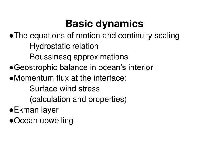
Basic dynamics ●The equations of motion and continuity scaling Hydrostatic relation Boussinesq approximations ●Geostrophic balance in ocean’s interior ●Momentum flux at the interface: Surface wind stress (calculation and properties) ●Ekman layer ●Ocean upwelling .

E N D
Basic dynamics ●The equations of motion and continuity scaling Hydrostatic relation Boussinesq approximations ●Geostrophic balance in ocean’s interior ●Momentum flux at the interface: Surface wind stress (calculation and properties) ●Ekman layer ●Ocean upwelling
The Equation of Motion Newton’s second law in a rotating frame.(Navier-Stokes equation) : Acceleration relative to axis fixed to the earth. : Pressure gradient force. : Coriolis force, where : Effective (apparent) gravity. : Friction. molecular kinematic viscosity.
Gravity: Equal Potential Surfaces • g changes about 5% 9.78m/s2 at the equator (centrifugal acceleration 0.034m/s2, radius 22 km longer) 9.83m/s2 at the poles) • equal potential surface normal to the gravitational vector constant potential energy the largest departure of the mean sea surface from the “level” surface is about 2m (slope 10-5) • The mean ocean surface is not flat and smooth earth is not homogeneous
Given the zonal momentum equation If we assume the turbulent perturbation of density is small i.e., The mean zonal momentum equation is Where Fx is the turbulent (eddy) dissipation If the turbulent flow is incompressible, i.e.,
Eddy Dissipation Reynolds stress tensor and eddy viscosity: , Then Where the turbulent viscosity coefficients are anisotropic. Ax=Ay~102-105 m2/s Az ~10-4-10-2 m2/s >>
Reynolds stress has no symmetry: A more general definition: if (incompressible)
Continuity Equation Mass conservation law In Cartesian coordinates, we have or For incompressible fluid, If we define and , the equation becomes
Scaling of the equation of motion • Consider mid-latitude (φ≈45o) open ocean away from strong current and below sea surface. The basic scales and constants: L=1000 km = 106 m H=103 m U= 0.1 m/s T=106 s (~ 10 days) 2Ωsin45o=2Ωcos45o≈2x7.3x10-5x0.71=10-4s-1 g≈10 m/s2 ρ≈103 kg/m3 Ax=Ay=105 m2/s Az=10-1 m2/s • Derived scale from the continuity equation W=UH/L=10-4 m/s
Scaling the vertical component of the equation of motion Hydrostatic Equation accuracy 1 part in 106
Boussinesq approximation Density variations can be neglected for its effect on mass but not on weight (or buoyancy). where , we have Assume that where Then the equations are (1) (2) where (3) (The term (4) is neglected in (1) for energy consideration.)
Pressure and Depth Hydrostatic pressure: where d is depth (instead of height) If we choose: ρ=1000 kg/m3 (2-4% lower than ρ of sea-water) g=10 m/s2 (2% higher than gravity) then p=1 decibar (db) is equivalent to 1 m of depth (p=1 db = 0.1 bar = 106 dyn/cm2 = 105 Pa (N/m2)) • True d is 1-2% less than the equivalent decibar depth.
Scaling of the horizontal components (accuracy, 1% ~ 1‰) Zero order (Geostrophic) balance Pressure gradient force = Coriolis force
Re-scaling the vertical momentum equation Since the density and pressure perturbation is not negligible in the vertical momentum equation, i.e., , and , The vertical pressure gradient force becomes
Taking into the vertical momentum equation, we have , and assume If we scale then and (accuracy ~ 1‰)
Geopotential Geopotential Φis defined as the amount of work done to move a parcel of unit mass through a vertical distance dz against gravity is The geopotential difference between levels z1 and z2 (with pressure p1 and p2) is (unit of Φ: Joules/kg=m2/s2).
Dynamic height , we have Given where is standard geopotential distance (function of p only) is geopotential anomaly. In general, Φ is sometime measured by the unit “dynamic meter” (1dyn m = 10 J/kg). which is also called as “dynamic height” (D) Units: δ~m3/kg, p~Pa, D~ dyn m Note: Though named as a distance, dynamic height (D) is still a measure of energy per unit mass.
Geopotential and isobaric surfaces Geopotential surface: constant Φ, perpendicular to gravitiy, also referred to as “level surface” Isobaric surface: constant p. The pressure gradient force is perpendicular to the isobaric surface. In a “stationary” state (u=v=w=0), isobaric surfaces must be level (parallel to geopotential surfaces). In general, an isobaric surface (dashed line in the figure) is inclined to the level surface (full line). In a “steady” state ( ), the vertical balance of forces is The horizontal component of the pressure gradient force is
Geostrophic relation The horizontal balance of force is where tan(i) is the slope of the isobaric surface. tan (i) ≈ 10-5 (1m/100km) if V1=1 m/s at 45oN (Gulf Stream). • In principle, V1 can be determined by tan(i). In practice, tan(i) is hard to measure because • p should be determined with the necessary accuracy • (2) the slope of sea surface (of magnitude <10-5) can not be directly measured (probably except for recent altimetry measurements from satellite.) (Sea surface is a isobaric surface but is not usually a level surface.)
Calculating geostrophic velocity using hydrographic data The difference between the slopes (i1 and i2) at two levels (z1 and z1) can be determined from vertical profiles of density observations. Level 1: Level 2: Difference: i.e., because A1C1=A2C2=L and B1C1-B2C2=B1B2-C1C2 because C1C2=A1A2 Note that z is negative below sea surface.
Since , and we have The geostrophic equation becomes
“Thermal Wind” Equation Starting from geostrophic relation Differentiating with respect to z Using Boussinesq approximation Or Rule of thumb: light water on the right. .
, The geostrophic current we calculate actually the “Thermal Wind” Analytically, or similarly
Since currents in deep ocean are much weak, there may exist a level (z2) where v1 >> v2 so that we can reasonably assume v2≈0 (level of no motion (LNM)). Then The rule for direction is the same for both p and ΔD. In practice, however, we see sections of hydrographic data (T, S, or σt). In that case, A rule for current direction is: (In northern hemisphere) Relative to the water below it, the current flows with the “lighter water on its right” In a vertical section, the isopycnals (curves of constant ρ or δ) slope downward from left to right. With respect to temperature, it is the “warmer water on its right”
Barotropic flow: p and ρ surfaces are parallel For a barotropic flow, we have is geostrophic current. Since Given a barotropic and hydrostatic conditions, and Therefore, And So
Baroclinic Flow: and There is no simple relation between the isobars and isopycnals. slope of isobar is proportional to velocity slope of isopycnal is proportional to vertical wind shear.
1½ layer flow Simplest case of baroclinic flow: Two layer flow of density ρ1 and ρ2. The sea surface height is η=η(x,y) (In steady state, η=0). The depth of the upper layer is at z=d(x,y). The lower layer is at rest. For z > d, For z ≤ d, If we assume The slope of the interface between the two layers (isopycnal)= times the slope of the surface (isobar). The isopycnal slope is opposite in sign to the isobaric slope.
Planetary boundary Layer near the sea surface: the effect of wind
Surface wind stress • Approaching sea surface, the geostrophic balance is broken, even for large scales. • The major reason is the influences of the winds blowing over the sea surface, which causes the transfer of momentum (and energy) into the ocean through turbulent processes. • The surface momentum flux into ocean is called the surface wind stress ( ), which is the tangential force (in the direction of the wind) exerting on the ocean per unit area (Unit: Newton per square meter) • The wind stress effect can be constructed as a boundary condition to the equation of motion as