Download
1 / 28
290 likes | 444 Views
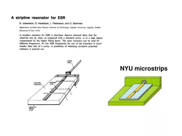
NYU microstrips. 1. Transmission mode TEM. only If b < /2 in our case 20 GHz, k = 12.9 ~ 2mm. Quasi-TEM mode. 2. Impedance Z. determined by the ratio / b and k. sample. L feed should be chosen to avoid resonance matching. Resonant frequencies.

E N D
1. Transmission mode TEM only If b < /2 in our case 20 GHz, k = 12.9 ~ 2mm Quasi-TEM mode 2. Impedance Z determined by the ratio /b and k
sample Lfeed should be chosen to avoid resonance matching Resonant frequencies l = 0.33b is a correction factor l n = 1 Half wavelength resonator fR = nf0 with n = 1,2,3…
ext Quality factor Q Internal (or unloaded) external (coupling to the external line)
f0 Familiar expression Q = f1-f2 f2 f1 f0 SOURCES OF ENERGY LOSS 1 - Ohmic losses: due to finite conductivity of the metal h substrate thickness skin depth (0.75m in aluminum at RT, decreases with T [factor 5, 4.2K]) Freq! Internal (or unloaded) quality factor Q0 Robert R. Romanovsky, NASA technical paper 2899 (1989) Analysis of microstrip resonators of titanium/gold and GaAs substrate Wallace and Silsbee, Rev. Sci. Instr., 62, 1754 (1991) Microstrip resonators for electron-spin resonance Due to Ohmic losses in the cavity and dielectric and radiation losses 2(energy stored) 2W Definition: Q = = P Energy loss/cicle 2 - Dielectric losses: due to finite conductivity of the dielectric dielectric constant conductivity of dielectric Negligible for GaAs!
CAVITY Discrete frequency-space available for photons resonances of the cavity 3 - radiation losses: due to radiation emitted. Resonator acts as an antenna These could be as important as the ohmic losses, especially at high frequency They can be avoided by shielding the resonator with a metallic cap! hf Continuous-frequency space available for photons
ALL CONTRIBUTIONS 4 – fringing fields: interection with layers outside the resonator perimeter These could also be important They can be minimized by etching oxide layers or covering the line! A is the area of the resonator L is the perimeter 2D is the conductivity of the external layer
ext External (or coupling) quality factor Qext Because the microwave resonator must be coupled to a transmission line for the measurements to be performed, the input impedance will be modified In general, the coupling between the resonator and the feed line contains resistive and reactive elements. This coupling loss component and the impedance of the transmission line load the resonator Therefore, the measured quality factor will differ from Q0 as: coupling coefficient d = 2k/(k+1) diameter of the reflection coefficient in the Smith chart d = 1 critically coupled d < 1 under coupled d > 1 over coupled QL = 2 Q0
Coupling to the coaxial also varies Q 1 - They adjust the coupling by inserting quartz rods in the holes of the gaps 2 – Tabib-Azar et al. (Rev. Sci. Instr., 70, 3083 (1999) They use EM simulation software to calculate the gap and they fine-tune the coupling with a dielectric piece over the feed line External (or coupling) quality factor Qext gap gap In our case the gap is much smaller ~ 100m also the quality factors are smaller Q ~ 40 - 100 No analytical expression to calculate the gap - Options:
Filling factor t is the sample thickness (assuming a thin-film) h is the substrate thickness Sensitivity = Q0 = t/ = 2 + a/b = 4 a a b Sample: a b TE101 resonant cavity Microstrip resonator Q0c(4K) = 2 Q0c(300K) = 10 Q0m(4K) = 5.5 Q0m(300K)
Electron Paramagnetic Resonance (EPR) measurements of high quality
NYU resonators stripline L w GaAs h • r = 12.9 (GaAs) • = 5.88107 s/m (copper) h = 0.5 mm
fres = 9.90 GHz Lfeed L w gap w GaAs h • r = 12.9 (GaAs) • = 5.88107 s/m (copper) h = 0.5 mm Lfeddline = 15.12 mm L = 4.82 mm w = 0.370 mm gap = 81.25 m Q ~ 500
fres = 15 GHz Lfeed L w gap w GaAs h • r = 12.9 (GaAs) • = 5.88107 s/m (copper) h = 0.5 mm Lfeddline = 9.77 mm L = 3 mm w = 0.381 mm gap = 102 m Q ~ 150
fres = 21.10 GHz Lfeed L w gap w GaAs h • r = 12.9 (GaAs) • = 5.88107 s/m (copper) h = 0.5 mm Lfeddline = 5.92 mm L = 2.0 mm w = 0.405 mm gap = 113.7 m Q ~ 100
fres = 26.08 GHz Lfeed L w gap w GaAs h • r = 12.9 (GaAs) • = 5.88107 s/m (copper) h = 0.5 mm Lfeddline = 4.98 mm L = 4.127 mm w = 0.432 mm gap = 107.4 m Q ~ 60
fres = 30.89 GHz Lfeed L w gap w GaAs h • r = 12.9 (GaAs) • = 5.88107 s/m (copper) h = 0.5 mm Lfeddline = 3.714 mm L = 1.15 mm w = 0.457 mm gap = 104.16 m Q ~ 1000? feed line = 11.42 mm
Transition 2.4 mm coaxial to microstrip Very small losses!
Results fres = 21.10 GHz Lfeed L w gap w GaAs h • r = 12.9 (GaAs) • = 5.88107 s/m (copper) h = 0.5 mm Lfeddline = 3 mm L = 2.0 mm Z ~ 35 + i15 w = 0.405 mm Complex input impedance gap = 113.7 m a dielectric over the feed line can improve Q Q ~ 100
1 2 fres = 21.10 GHz Lfeed L w gap w GaAs h • r = 12.9 (GaAs) • = 5.88107 s/m (copper) h = 0.5 mm Lfeddline = 3 mm L = 2.0 mm w = 0.405 mm gap = 113.7 m Q ~ 100
3 fres = 21.10 GHz Lfeed L w gap w GaAs h • r = 12.9 (GaAs) • = 5.88107 s/m (copper) h = 0.5 mm Lfeddline = 3 mm L = 2.0 mm w = 0.405 mm gap = 113.7 m Q ~ 100
3 fres = 21.10 GHz Lfeed L w gap
4 fres = 21.10 GHz Lfeed L w gap w GaAs h • r = 12.9 (GaAs) • = 5.88107 s/m (copper) h = 0.5 mm Lfeddline = 3 mm L = 2.0 mm w = 0.405 mm gap = 113.7 m Q ~ 100
fres = 21.10 GHz Lfeed L w gap w GaAs h • r = 12.9 (GaAs) • = 5.88107 s/m (copper) h = 0.5 mm Lfeddline = 3 mm L = 2.0 mm w = 0.405 mm gap = 113.7 m Q ~ 100
fres = 15 GHz Lfeed L w gap w GaAs h • r = 12.9 (GaAs) • = 5.88107 s/m (copper) h = 0.5 mm Lfeddline = 9.77 mm L = 3 mm w = 0.381 mm gap = 102 m Q ~ 150
fres = 9.90 GHz Lfeed L w gap w GaAs h • r = 12.9 (GaAs) • = 5.88107 s/m (copper) h = 0.5 mm Lfeddline = 15.12 mm L = 4.82 mm w = 0.370 mm gap = 81.25 m Q ~ 500