Download
1 / 22
220 likes | 526 Views
Lecture 7. Markov Model with Matrixes. Introduction to HMM with the example of DNA analysis. Distributions. Probability density and cumulative distribution functions. Poisson and Normal distributions. Practice: Distributions with Mathematica.

E N D
Lecture 7.Markov Model with Matrixes. Introduction to HMM with the example of DNA analysis.Distributions. Probability density and cumulative distribution functions.Poisson and Normal distributions.Practice: Distributions with Mathematica
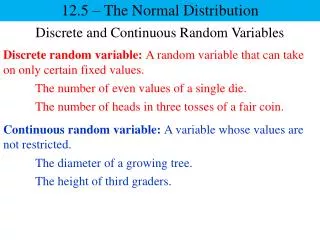
7.1 ReminderWe remind here some facts about the distributions of discrete and continuous random variables. The discrete random distribution can be characterized by a probability function p(xi) assigning the probabilities to all possible values xi of a random variable X. The probability function should satisfy the following equations : Compare with the pages 31 … of Lect. 1
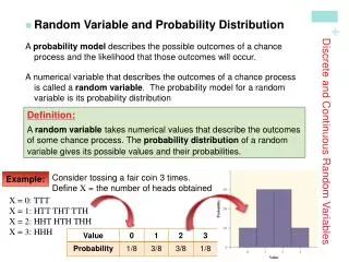
Example: Suppose that a coin is tossed twice, so that the sample space is ={HH,HT,TH,TT}. Let X represent a number of heads that can come up. Find the probability function p(x). As we know, the probability function is thus given by the table: The graphical example presented below represents a typical way of depicting the probability distribution for a discrete random variable
~p(xi) 0.3 1 2 3 4 5 6 7 8 9 10 11 Possible values of the random variable, xi
Continuous distribution. Probability density function (PDF). Remember: For a continuous variable we must assign to each outcome a probability p(x )=0. Otherwise, we would not be able to fulfill the requirement 7.1 (the second of three). A random variable X is said to have a continuous distribution with density functionf(x) if for all a b we have The analogs of Eqs. 7.2 and 7.3 for the continuous distributions would be
P(E) is a probability that X belongs to E. f(x) P(a<X<b) a b Geometrically, P(a<X<b) is the area under the curve f(x) between a and b. The question: Can f(x) exceed 1? Please argue.
7.2 A few new distributions and their properties a. Poission distributionPoisson distribution is one of the most important discrete distributions. Its probability function is Poisson distribution is a limiting case of the Binomial distribution P(pn,n), with parameters pnand n such that In other words, if we have a large number of independent events with small probability, then number of occurrences has approximately Poisson distribution. Let us introduce now a more intuitive definition of the Poisson distribution.
Examples with Poisson distribution 1. Suppose that the probability of a defect in a foot of magnetic tape is 0.002. Use the Poisson distribution to compute the probability that 1500 feet roll will have no defects .
This example helps to describe the Poisson Distribution in a new way by noticing that is the expected (average) value of the defects in 1500 feet of the tape. In other words, the PD gives the probability of n events happening in some experiment if the expected (average) number of the events, , for this particular experiment, is known. Attention: it is important to understand that is the average (expected) value for the interval (of time, or space) where the n questioned events should occur. For instance, in the former example is the average value of defects per 1500 feet of tape (but not per a foot, or per 1000 feet, etc).
Example 2 An airline company sells 200 tickets for a plane with 198 seats, knowing that a probability that a passenger will not show up for the flight is 0.008. Use the Poisson approximation to compute the probability that they will have enough seats for all the passengers that will show up.
Solution. p=0.012, L=0.012*200=2.4 – the average number (out of 200 passengers ) that won’t show up for the flight. p[x]= Exp[-2.4]2.4x/x!; P[more than 1 person won’t show up] = 1-p[0]-p[1]= ~ 0.7. In other words, there is (only) a 30% of chance that they more than 198 passengers will show up. This is quite a familiar scenario: the company would typically offer you a free additional ticket for a future flight if you agree on switching to a later flight.
Example 3: (working in groups) 10% of the tools produced in a certain manufacturing process turns out to be defective. Find a probability that in a sample of ten tools selected at random, exactly 2 will be defective, by using (a) binomial and (b) Poisson distribution. Open a Mathematica file, and find the probabilities
b. The exponential distribution (this is the continuous distribution, for the continuous random variable x). Those who know how to integrate can verify that (7.8) satisfies (7.5) (the total area under the curve f(x) equals 1. Note: In Matematica, the integral of a function f[x] can be found as: Integrate[f[x],{x,x1,x2}] , Shift+Enter. Here x1and x2 are the limits of integration.
A typical example of the exponential distribution results from the discussion of the waste products of the nuclear power plant. If at time t=0 there are N(0) identical unstable particles, and the number of particles dN(t) decaying in time dt is proportional to dt and to the number of particles, then we have dN(t)= - N(t)dt This is so called differential equation. Here is how it is solved with Mathematica. DSolve[{n’[t] + G n[t] == 0, n[0] == n0},n[t],t]; n[t]-> n0 Exp[-Gt]; As a result we came up with the exponential distribution.
Let’s introduce the “half-time” T , such that N(T)=N0/2. Then we find: T=ln2=0.693. c. The standard normal distribution f(x)=(2)-1/2 exp(-x2/2) (7.12) A. Using Mathematica, check that this PDF satisfies the normality condition (7.5). Make a plot of (7.12). If a random variable y is related to x as y=ax+b, how the distribution function f(y) looks like? (we assume that x is distributed according to (7.12).
More generally, X is said to have a normal (,2) distribution if it has density function f(x)=(2 2)-1/2 exp[-(x- )2/2 2] (7.12’) 2 is called “variance” and is the “mean” or the “expectation”. Try to analyze, assigning different numeric values to and 2 how they affect the shape of f(x). For instance, how the parameters for the green and red curves are related? Green and blue? See the Mathematica file
7.3 Probability distribution function( also called “cumulative distribution function”= CDF) 1. Continuous random variable From the “outside”, random distributions are well described by the probability distribution function (we will use CDF for short) F(x) defined as This formula can also be rewritten in the following very useful form: Question: Can F(x) exceed 1? Argue it.
To see what the distribution functions look like, we return to our examples. 1. The uniform distribution (7.7): Using the definition (7.13) and Mathematica, try to find F(x) for the uniform distribution. Prove thatF(x)=0 for x a; (x-a)/(b-a) for a x b; 1 for x>b. Draw the CDF for several a and b. Consider an important special case a=0, b=1. How is it related tothe spinner problem? To the balanced die? 2. The exponential distribution (7.8):
Use Mathematica to prove that F(x)= 0 for x 0; 1-exp(-x) for x >0. (7.15) “Lack of memory” for the exponential distribution Suppose that X has an exponential distribution (7.8). The probability that the event (such as the radioactive decay) did not happen in t units of time is P(X>t) = 1-F(x). According to (7.15) it results in P(X>t)= exp(-t) . Let’s find now a probability that we will have to wait some additional time s given that we have been waiting t units of time: P(X>t+s|T>t) = P(X > t+s)/P(X > t) = exp[-(t+s)]/ exp[-t)]= exp[-s]. As we see, the result depends only on s and does not depend on the previous waiting time. The probability you must wait additional s units of time till decay occurs is the same as if you had not been waiting at all.
The standard normal distribution Using Mathematica and Eq. (7.12), find F[x] for the snd. Use NIntegrate[f[t],{t,-,x}] and Plot[…] functions. 2. CDF for discrete random variables For discrete variables the integration is substituted for summation: It is clear from this formula that if X takes only a finite number of values, the distribution function looks like a stairway.
F(x) p(x4) 1 p(x3) p(x2) p(x1) x1 x2 x3 x4 x Draw F(x) for the example in page 7.
This problem is for your practice Predicting the rate of mutation based on the Poisson probability distribution function. The evolutionary process of amino acid substitutions in proteins is