Download
1 / 47
560 likes | 877 Views
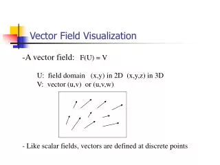
Vector Field Visualization. * T. Moeller, H. Shen 의 slide 를 이용함. Vector Field Visualization. A vector field: F(U) = V U: field domain (x,y) in 2D (x,y,z) in 3D V: vector (u,v) or (u,v,w) - Like scalar fields, vectors are defined at discrete points.

E N D
Vector Field Visualization * T. Moeller, H. Shen 의 slide를 이용함.
Vector Field Visualization • A vector field: F(U) = V • U: field domain (x,y) in 2D (x,y,z) in 3D • V: vector (u,v) or (u,v,w) • - Like scalar fields, vectors are defined at discrete points
Flow Visualization • Flow visualization – classification – Dimension (2D or 3D) – Time-dependency: steady vs. unsteady – Grid type
Examples • http://hint.fm/wind/
Vector Field Visualization Challenges • General Goal • Display the field’s directional information • Domain Specific • Detect certain features • e.g. vortex cores
Vector Field Visualization Challenges • A good vector field visualization is difficult to get: • Displaying a vector requires more visual attributes (u,v,w): direction and magnitude • Displaying a vector requires more screen space • more than one pixel is required to display an arrow => It becomes more challenging to display a dense vector field
Vector Field Visualization Techniques • Local technique • Particle Advection • Display the trajectory of a particle starting from a particular location • Global technique • Hedgehogs, Line Integral Convolution etc • Display the flow direction everywhere in the field
Characteristic of Lines • Streamline • tangential to the vector field • Pathline • trajectories of massless particles in the flow • Streakline • trace of dye that is released into the flow at a fixed position • Time line (Time surface) • propagation of a line (surface) of massless elements in time Streamline, pathline and streakline are different only when the flow is unsteady (time dependent)
Streaklines • Trace of dye that is released into the flow at a fixed position • Connect all particles that passed through a certain position
Time lines (Time surfaces) • Propagation of a line (surface) of massless elements in time • Idea: “consists” of many point-like particles that are traced • Connect particles that were released simultaneously t0 t1 t2 Timelines or time surfaces can show the evolution of a flow.
Example :streamline, pathline, streakline The red particle moves in a flowing fluid; Its pathline is traced in red; the tip of the trail of blue ink released from the origin follows the particle, but unlike the static pathline (which records the earlier motion of the dot), ink released after the red dot departs continues to move up with the flow. (This is a streakline.) The dashed lines represent contours of the velocity field (streamlines), showing the motion of the whole field at the same time.
Stream ball • Use radii to visualize additional properties (e.g. divergence and acceleration in a flow)
Stream ribbons • The area swept out by a deformable line segment along a streamline • Visualizes rotational behavior of a 3D flow
streamtubes • Thick tube shaped streamline whose radial extent shows the expansion of flow
Local technique - Particle Tracing Visualizing the flow directions by releasing particles and calculating a series of particle positions based on the vector field The motion of particle: dx/dt = v(x) x: particle position (x,y,z) v(x): the vector (velocity) field Use numerical integration to compute a new particle position x(t+dt) = x(t) + Integration( v(x(t)) dt )
Numerical Integration First Order Euler method: x(t+dt) = x(t) + v(x(t)) * dt - Not very accurate, but fast - Other higher order methods are available: Runge-Kutta second and fourth order integration methods (more popular due to their accuracy) Result of first order Euler method
x(t+dt) x(t) ½ * [v(x(t))+v(x(t)+dt*v(x(t))] Numerical Integration (2) Second Runge-Kutta Method x(t+dt) = x(t) + ½ * (K1 + K2) k1 = dt * v(x(t)) k2 = dt * v(x(t)+k1)
Numerical Integration (3) Standard Method: Runge-Kutta fourth order x(t+dt) = x(t) + 1/6 (k1 + 2k2 + 2k3 + k4) k1 = dt * v(t); k2 = dt * v(x(t) + k1/2) k3 = dt * v(x(t) + k2/2); k4 = dt * v(x(t) + k3)
Streamline • Displaying streamlines is a local technique because you can only visualize the flow directions initiated from one or a few particles • When the number of streamlines is increased, the scene becomes cluttered • You need to know where to drop the particle seeds • Streamline computation is expensive
Arrows and Glyphs • Visualize local features of the vector field: • Vector itself • Extern data: temperature, pressure, etc. • Important elements of a vector: • Direction • Magnitude • Not: components of a vector • Approaches: • Arrow plots • Glyphs
Arrows • Arrows visualize • Direction of vector filed • Magnitude • Length of arrows • Color coding
Glyphs • Can visualize more features of the vector field
Flow Volume • Construction of the flow volume • Seed polygon (square) is used as smoke generator • Constrained such that center is perpendicular to flow • Square can be subdivided into a finer mesh • Volume rendering • Opacity is inversely proportional to the tetrahedra’s volume
Global Techniques • Display the entire flow field in a single picture • Minimum user intervention • Example: Hedgehogs (global arrow plots)
LIC : Line Integral Convolution • Given : • Vector field and texture image • Texture image is normally white noise • Output • Colored field correlated in the flow direction Convolve a random texture along the streamlines
LIC • Visualize dense flow fields by imaging its integral curves • Cover domain with a random texture (so called ‚input texture‘, usually stationary white noise) • Blur (convolve) the input texture along the path lines using a specified filter kernel
LIC : Idea • Global visualization technique • Dense representation • Start with random texture • Smear out along stream lines
OLIC : Oriented Line Integral Convolution • Visualizes orientation (in addition to direction) • Use • Sparse texture • Anisotropic convolution kernel
세부적인 이슈 소개 • Illumination • Seed Placement
Comparisons Fully opaque Use transparency With Illumination
Seed Placement for Streamline • The placement of seeds directly determines the visualization quality • Too many: scene cluttering • Too little: no pattern formed • It has to be the right number at the right places!!!
Image-Guided Streamline Placement • Main idea: the distribution of ink on the screen should be even [turk 96]
2 S S (L*I (x,y) - t ) x y Use Energy Function as a Metric • An energy function is defined to measure whether ‘ink’ is distributed evenly • I(x,y): image with streamlines • L: A low pass filter (Gaussian or Hermit interpolation) • t: A user specified threshold for average image intensity
Iterative Algorithm • Place an initial set of seeds and compute streamlines • Iteratively minimize the energy function (random decent) with the following operations on the seeds: • Move • Insert • Delete • Lengthen • Shorten • Combine • Iterate until the energy function converges
Results After energy minimization Seeds at regular grid