Download
1 / 23
240 likes | 537 Views
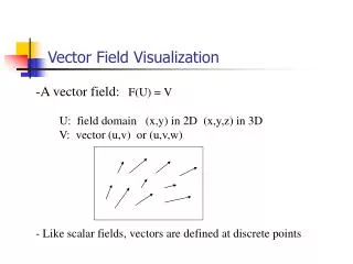
Vector Field Visualization. A vector field: F(U) = V U: field domain (x,y) in 2D (x,y,z) in 3D V: vector (u,v) or (u,v,w) - Like scalar fields, vectors are defined at discrete points. Vector Field Viz Applications. Computational Fluid Dynamics. Weather modeling.

E N D
Vector Field Visualization • A vector field: F(U) = V • U: field domain (x,y) in 2D (x,y,z) in 3D • V: vector (u,v) or (u,v,w) • - Like scalar fields, vectors are defined at discrete points
Vector Field Viz Applications Computational Fluid Dynamics Weather modeling
Vector Field Visualization Challenges General Goal: Display the field’s directional information Domain Specific: Detect certain features Vortex cores, Swirl
Vector Field Visualization Challenges A good vector field visualization is difficult to get: - Displaying a vector requires more visual attributes (u,v,w): direction and magnitude - Displaying a vector requires more screen space more than one pixel is required to display an arrow ==> It becomes more challenging to display a dense vector field
Vector Field Visualization Techniques Local technique:Particle Advection - Display the trajectory of a particle starting from a particular location Global technique: Hedgehogs, Line Integral Convolution, Texture Splats etc - Display the flow direction everywhere in the field
Local technique - Particle Tracing Visualizing the flow directions by releasing particles and calculating a series of particle positions based on the vector field The motion of particle: dx/dt = v(x) x: particle position (x,y,z) v(x): the vector (velocity) field Use numerical integration to compute a new particle position x(t+dt) = x(t) + Integration( v(x(t)) dt )
Numerical Integration First Order Euler method: x(t+dt) = x(t) + v(x(t)) * dt - Not very accurate, but fast - Other higher order methods are avilable: Runge-Kutta second and fourth order integration methods (more popular due to their accuracy) Result of first order Euler method
x(t+dt) x(t) ½ * [v(x(t))+v(x(t)+dt*v(x(t))] Numerical Integration (2) Second Runge-Kutta Method x(t+dt) = x(t) + ½ * (K1 + K2) k1 = dt * v(x(t)) k2 = dt * v(x(t)+k1)
Numerical Integration (3) Standard Method: Runge-Kutta fourth order x(t+dt) = x(t) + 1/6 (k1 + 2k2 + 2k3 + k4) k1 = dt * v(t); k2 = dt * v(x(t) + k1/2) k3 = dt * v(x(t) + k2/2); k4 = dt * v(x(t) + k3)
Streamlines A curves that connect all the particle positions
Streamlines (cont’d) - Displaying streamlines is a local technique because you can only visualize the flow directions initiated from one or a few particles - When the number of streamlines is increased, the scene becomes cluttered - You need to know where to drop the particle seeds - Streamline computation is expensive
T=3 T=4 T=2 T=5 timeline T = 2 T = 1 T = 3 Pathlines, Timelines, and Streaklines • Extension of streamlines for time-varying data • Pathlines: • Timelines: T=1
b.t. =1 b.t. =2 b.t. =3 b.t. =4 b.t. =5 Streaklines - Continuously injecting a new particle at each time step, advecting all the existing particles and connect them together into a streakline
Global techniques - Display the entire flow field in a single picture - Minimum user intervention - Example: Hedgehogs (global arrow plots)
Hedgehogs - Dense 2D fields or 3D fields are difficult
More global techniques Texture Splats