Download
1 / 89
930 likes | 1.11k Views
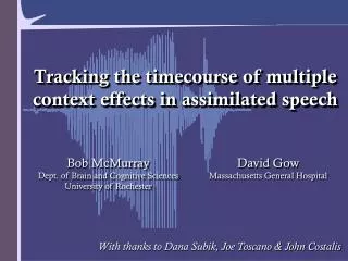
Tracking the time course of lexical access in continuous speech. Michael K. Tanenhaus Department of Brain and Cognitive Sciences Department of Linguistics University of Rochester. Collaborators. Jim Magnuson Columbia University Delphine Dahan Anne Pier Salverda

E N D
Tracking the time course of lexical access in continuous speech Michael K. Tanenhaus Department of Brain and Cognitive Sciences Department of Linguistics University of Rochester
Collaborators Jim Magnuson Columbia University Delphine Dahan Anne Pier Salverda Max Planck Institute for Psycholinguistics Dick Aslin Katherine Crosswhite Joyce McDonough Bob McMurray Mikhail Masharov University of Rochester
Overview Why use eye movements to study speech? Basic results and a linking hypothesis: time course of rhyme and cohort effects linking hypothesis to fixations The closed set problem: lexicality and subcategorical mismatch mapping from speech to pictures A new look at some classic issues: Time course of neighborhood effects VOT and lexical access Effects of prosodic domains on lexical neighborhoods Semantic context and lexical access
Macrostructure vs Microstructure Macrostructure: • Properties of system compatible with some broad classes of models but not others • Informal models • Rough linking hypotheses between models and measures (rejecting) null hypothesis experiments often sufficient Microstructure: • Specific mechanisms with detailed representational and processing assumptions • Quantitative models • Explicit linking hypotheses • Goodness of fit experiments typically required
Macrostructure of spoken word recognition Word recognition takes place against a backdrop of dynamically changing partially activated lexical candidates that compete for recognition
Importance of time course • Many theoretical issues about microstructure hinge on time course • Quantitative models make detailed time course predictions • Conventional measures don’t address time course naturally • Interrupt speech (gating) • Require metalinguistic decision (lexical decision) • More complex than current models (cross-modal priming) • How does activation map quantitatively onto priming? • Need fine-grained time-course measure with an explicit linking hypothesis.
Why Eye movements? • closely time-locked to speech • ballistic measure • can be used with continuous speech • natural response measure • low threshold response • subject is unaware • does not require meta-linguistic judgment • plausible linking hypothesis: Probability of eye movement at time (t)is a function of activation of possible alternatives plus some constant for programming and execution (~200ms)
Allopenna, Magnuson & Tanenhaus (JML, 1998) • Does the competitor set include lexical candidates that have mismatching onsets? • e.g., does beaker activate “speaker” • Evaluate linking hypothesis between activation in an explicit continuous mapping model, TRACE, and a response measure, fixations.
TRACE activation functions for target, cohort, rhyme and unrelated competitors
Allopenna, Magnuson & Tanenhaus (1998) Eye Eye camera tracking computer Scene camera ‘Pick up the beaker’
Fixation Proportions over Time Trials 1 2 3 4 5 Time 200 ms Proportion of fixations Time + Target = beaker Cohort = beetle Unrelated = carriage Look at the cross. Click on the beaker.
Fixation Proportions summed over an interval Trials 1 2 3 4 5 Proportion of fixations Proportion of fixations cohort Time unrelated +
Fixation time over an interval Trials 1 2 3 4 5 Proportion of fixations Time + Time spent fixating (ms) cohort unrelated
Allopenna, Magnuson & Tanenhaus (1998) Eye Eye camera tracking computer Scene camera ‘Pick up the beaker’
•Activation converted to probabilities using the Luce (1959) choice rule • Si = e kai • S: response strength for each item • a: activation • k: free parameter, determines amount of separation between activation levels (set to 7) • Li = Si / ∑ Si • Choice rule assumes each alternative is equally probable given no information; when initial instruction is “look at the cross” or look at picture X, we scale the response probabilities to be proportional to the amount of activation at each time step: • di = max_acti / max_act_overall • Ri = di Li Referent (e.g., "beaker") Cohort (e.g., "beetle") Rhyme (e.g., "speaker") Unrelated 0 200 400 600 800 1000 Time since target onset (msec) Linking hypothesis
The closed set problem Aunt Tillie’s Umbrella
camera beagle beast bead beak carriage speaker beaker beetle Will we see effects of non-displayed, non-pictured candidates?
X-spliced stimuli with misleading coarticulatory information • NE(t)T (word from itself) • (net cross-spliced using the onset and vowel from another token of net) • NE(k)T (word from another word) • (net cross-spliced using the onset and vowel from neck) • NE(p)T (word from a nonword) • (net cross-spliced using the onset and vowel from nep) Dahan, Magnuson, Tanenhaus & Hogan, LCP, 2001
Lexical competitor not mentioned or displayed ne(k)t ne(p)t ne(t)t Click on the
camera beagle beast bead beak neck ring bell lobster net Prediction: Delayed target looks to the net with NE(k)T compared to NE(p)T
NE(p)T NE(k)T We see an effect of lexical status indicating that activation is affected by the full lexicon
snake How can people look at the referent so quickly? Assumption: Lexical representations include perceptual/conceptual information that is activated from earliest moments of lexical access Is it because they are naming the pictures? Prediction: Early fixations should show “visual” competitor effects Would not predict this if people were naming the pictures
Dahan and Tanenhaus (in preparation) How materials were constructed: (1) non-prototypical* picture of target (2) visual competitor similar to prototype* * DD-Prototypes
Participants heard the name of the target picture in isolation (e.g., “slang”, snake) • 300 ms of pre-exposure
Results 300 ms
Conclusions Eye movements provide a sensitive measure of the time course of lexical activation that is sensitive to fine-grained phonetic/acoustic variation in the signal. Linking hypothesis between fixations and lexical representations seems plausible. Very early access to lexically-based perceptual/conceptual information.
New look at classic issues • Time course of competitor effects • (Magnuson, Tanenhaus & Aslin, in preparation) • VOT and lexical access • Prosodic domains and lexical neighborhoods • Semantic context and lexical access
Time course of competitor effects • We know cohorts and rhymes have different time courses • What are the implications for global metrics like neighborhood? • Manipulate: • Word frequency • Neighborhood density • Cohort density • Examine time course
High Frequency Low Frequency High NB Low NB High NB Low NB High Cohort 16 16 High Cohort 16 16 Low Cohort 16 16 Low Cohort 16 16 Low High Log frequency 2.3 4.7 Neighborhood density 26.0 101.5 Cohort density 47.3 289.0 Materials
Procedure • 15 participants • 4 items displayed (Allopenna et al. procedure) • Displayed items phonologically and semantically unrelated • Instruction: “Click on the fox.” • Dependent measure: fixation proportion to targets over time • Predictions: • High frequency faster than low frequency • Low neighborhood faster than high • Low cohort faster than high • Stats: ANOVAs on mean fixation proportion from 200 ms to 1000 ms
New look at classic issues • Time course of competitor effects • VOT and lexical access • (McMurray, Tanenhaus & Aslin, 2002) • Prosodic domains and lexical neighborhoods • Semantic context and lexical access
McMurray, Tanenhaus & Aslin, 2002 Effects of within-category VOT on lexical access
B Discrimination ID (%/pa/) P • Sharp identification of speech sounds on a continuum • Discrimination poor within a phonetic category Categorical Perception Listeners are NOT sensitive to small VOT differences. 100 % /p/ 0 B VOT P
Experiment 1: Categorical Perception B P Ba 1 2 3
Experiment 1: Identification Results 1 0.9 0.8 0.7 0.6 0.5 0.4 0.3 0.2 0.1 0 0 5 10 15 20 25 30 35 40 Category Boundary 17.5 +/- .83ms Proportion of /p/ response B P VOT (ms) Steep ID function characteristic of Categorical Perception.Stimuli are good.
Lexical Identification Six 9-step /ba/ - /pa/ VOT continuum (0-40ms) Bear/Pear Beach/Peach Butter/Putter Bale/Pale Bump/Pump Bomb/Palm 12 L- and Sh- Filler items Leaf Lamp Ladder Lock Lip Leg Shark Ship Shirt Shoe Shell Sheep Identification indicated by mouse click on picture Eye movements monitored at 250 hz 17 Subjects
Lexical Identification A moment to view the items
Lexical Identification 500 ms later
Identification Results 1 0.9 0.8 0.7 0.6 Yields a “perfect” categorization function. 0.5 0.4 0.3 0.2 0.1 0 0 5 10 15 20 25 30 35 40 ID Function after filtering Actual Exp2 Data Trials with low-frequency response excluded. proportion /p/ B VOT (ms) P
Categorical? 0.08 0.07 0.06 0.05 Andruski et al (schematic) Gradient Sensitivity 0.04 “Categorical” Perception 0.03 0.02 0 5 10 15 20 25 30 35 40 Looks to Looks to Fixation proportion VOT (ms)
20 ms 25 ms 30 ms 10 ms 15 ms 35 ms 40 ms 0.16 0.14 0.12 0.1 0.08 0.06 0.04 0.02 0 0 400 800 1200 1600 0 400 800 1200 1600 2000 Eye Movement Results Gradient effects of VOT? Response= Response= VOT VOT 0 ms 5 ms Fixation proportion Time since word onset (ms)
0.08 0.07 0.06 0.05 0.04 0.03 0.02 0 5 10 15 20 25 30 35 40 Competitor looks as function of VOT Response= Response= Looks to Fixationproportion Looks to Category Boundary VOT (ms)
0.08 0.07 0.06 0.05 0.04 0.03 0.02 0 5 10 15 20 25 30 35 40 Clear effects of VOT B: p=.017* P: p<.0001*** Linear Trend B: p=.023* P: p=.002** Linear Trend even when boundary VOTs excluded Response= Response= Looks to Fixation proportion Looks to Category Boundary VOT (ms) Unambiguous Stimuli Only
Lexical sensitivity to subphonemic variation Why would lexical sensitivity to subphonemic differences be a good idea? • Extract more information from the signal • Position in a Prosodic domain affects consonants • Strong position in a prosodic domain characterized by: • Longer VOTs • Hyper-articulation (more extreme formant transitions) • Burst amplitude • Could be used to help resolve temporary phonetic/lexical ambiguities when subsequent information arrives (e.g. vowel length or sentential context)
New look at classic issues • Time course of competitor effects • VOT and lexical access • Prosodic domains and lexical neighborhoods • (Salverda et al., in preparation) • Semantic context and lexical access