Chapter 3: Pulse Code Modulation

1. Chapter 3:Pulse Code Modulation • Pulse Code Modulation • Quantizing • Encoding • Analogue to Digital Conversion • Bandwidth of PCM Signals Huseyin Bilgekul Eeng360 Communication Systems I Department of Electrical and Electronic Engineering Eastern Mediterranean University

2. PULSE CODE MODULATION (PCM) • DEFINITION: Pulse code modulation (PCM) is essentially analog-to-digital conversion of a special type where the information contained in the instantaneous samples of an analog signal is represented by digital words in a serial bit stream. • The advantages of PCM are: • Relatively inexpensive digital circuitry may be used extensively. • PCM signals derived from all types of analog sources may be merged with data signals and transmitted over a common high-speed digital communication system. • In long-distance digital telephone systems requiring repeaters, a clean PCM waveform can be regenerated at the output of each repeater, where the input consists of a noisy PCM waveform. • The noise performance of a digital system can be superior to that of an analog system. • The probability of error for the system output can be reduced even further by the use of appropriate coding techniques.

3. Sampling, Quantizing, and Encoding • The PCM signal is generated by carrying out three basic operations: • Sampling • Quantizing • Encoding • Sampling operation generates a flat-top PAM signal. • Quantizing operation approximates the analog values by using a finite number of levels. This operation is considered in 3 steps • Uniform Quantizer • Quantization Error • Quantized PAM signal output • PCM signal is obtained from the quantized PAM signal by encoding each quantized sample value into a digital word.

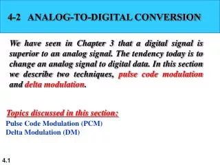
4. 111 110 101 100 011 010 001 000 Digital Output Signal 111 111 001 010 011 111 011 Analog to Digital Conversion • The Analog-to-digital Converter (ADC) performs three functions: • Sampling • Makes the signal discrete in time. • If the analog input has a bandwidth of W Hz, then the minimum sample frequency such that the signal can be reconstructed without distortion. • Quantization • Makes the signal discrete in amplitude. • Round off to one of q discrete levels. • Encode • Maps the quantized values to digital words that are bits long. • If the (Nyquist) Sampling Theorem is satisfied, then only quantization introduces distortion to the system. Analog Input Signal Sample ADC Quantize Encode

5. Quantization • The output of a sampler is still continuous in amplitude. • Each sample can take on any value e.g. 3.752, 0.001, etc. • The number of possible values is infinite. • To transmit as a digital signal we must restrict the number of possible values. • Quantization is the process of “rounding off” a sample according to some rule. • E.g. suppose we must round to the nearest tenth, then: • 3.752 --> 3.8 0.001 --> 0

6. Illustration of the Quantization Error

7. PCM TV transmission: • 5-bit resolution; • 8-bit resolution.

8. Dynamic Range: (-8, 8) Output sample XQ 7 5 3 1 -8 -6 8 -4 -2 2 4 6 -1 -3 -5 -7 Quantization Characteristic Uniform Quantization • Most ADC’s use uniform quantizers. • The quantization levels of a uniform quantizer are equally spaced apart. • Uniform quantizers are optimal when the input distribution is uniform. When all values within the Dynamic Range of the quantizer are equally likely. Input sample X Example: Uniform  =3 bit quantizer q=8 and XQ = {1,3,5,7}

9. Quantization Example Analogue signal Sampling TIMING Quantization levels. Quantized to 5-levels Quantization levels Quantized 10-levels

10. PCM encoding example Levels are encoded using this table Table: Quantization levels with belonging code words M=8 Chart 2. Process of restoring a signal. PCM encoded signal in binary form: 101 111 110 001 010 100 111 100 011 010 101 Total of 33 bits were used to encode a signal Chart 1. Quantization and digitalization of a signal. Signal is quantized in 11 time points & 8 quantization segments.

11. Encoding • The output of the quantizer is one of M possible signal levels. • If we want to use a binary transmission system, then we need to map each quantized sample into an n bit binary word. • Encoding is the process of representing each quantized sample by an  bit code word. • The mapping is one-to-one so there is no distortion introduced by encoding. • Some mappings are better than others. • A Gray code gives the best end-to-end performance. • The weakness of Gray codes is poor performance when the sign bit (MSB) is received in error.

12. Gray Codes • With gray codes adjacent samples differ only in one bit position. • Example (3 bit quantization): XQ Natural coding Gray Coding +7 111 110 +5 110 111 +3 101 101 +1 100 100 -1 011 000 -3 010 001 -5 001 011 -7 000 010 • With this gray code, a single bit error will result in an amplitude error of only 2. • Unless the MSB is in error.

13. Waveforms in a PCM system for M=8 M=8 (a) Quantizer Input output characteristics (b) Analog Signal, PAM Signal, Quantized PAM Signal (c) Error Signal (d) PCM Signal

14. PCM Transmission System

15. Practical PCM Circuits • Three popular techniques are used to implement the analog-to-digital converter (ADC) encoding operation: • The counting or ramp, ( Maxim ICL7126 ADC) • Serial or successive approximation, (AD 570) • Parallel or flash encoders. ( CA3318) • The objective of these circuits is to generate the PCM word. • Parallel digital output obtained (from one of the above techniques) needs to be serialized before sending over a 2-wire channel • This is accomplished by parallel-to-serial converters [Serial Input-Output (SIO) chip] • UART,USRT and USART are examples for SIO’s

16. Bandwidth of PCM Signals • The spectrum of the PCM signal is not directly related to the spectrum of the input signal. • The bandwidth of (serial) binary PCM waveforms depends on the bit rate R and the waveform pulse shape used to represent the data. • The Bit Rate R is R=nfs Where n is the number of bits in the PCM word (M=2n) and fsis the sampling rate. • For no aliasing case (fs≥ 2B), the MINIMUM Bandwidth of PCM Bpcm(Min) is: Bpcm(Min)= R/2 = nfs//2 The Minimum Bandwidth of nfs//2 is obtained only when sin(x)/x pulse is used to generate the PCM waveform. • For PCM waveform generated by rectangular pulses, the First-null Bandwidth is: Bpcm= R = nfs