Download
1 / 16
180 likes | 902 Views
Prof. Brian L. Evans Dept. of Electrical and Computer Engineering The University of Texas at Austin. Quadrature Amplitude Modulation (QAM) Transmitter. Introduction. Digital Pulse Amplitude Modulation (PAM) Modulates digital information onto amplitude of pulse

E N D
Prof. Brian L. Evans Dept. of Electrical and Computer Engineering The University of Texas at Austin Quadrature Amplitude Modulation (QAM) Transmitter
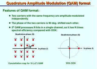
Introduction • Digital Pulse Amplitude Modulation (PAM) Modulates digital information onto amplitude of pulse May be later upconverted (e.g. to radio frequency) • Digital Quadrature Amplitude Modulation (QAM) Two-dimensional extension of digital PAM Baseband signal requires sinusoidal amplitude modulation May be later upconverted (e.g. to radio frequency) • Digital QAM modulates digital information onto pulses that are modulated onto Amplitudes of a sine and a cosine, or equivalently Amplitude and phase of single sinusoid
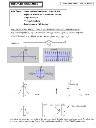
Review Y1(w) ½X1(w + wc) ½X1(w - wc) X1(w) ½ 1 w -wc - w1 -wc + w1 wc - w1 wc + w1 0 -wc wc w -w1 w1 0 Amplitude Modulation by Cosine • y1(t) = x1(t) cos(wct) Assume x1(t) is an ideal lowpass signal with bandwidth w1 Assume w1 << wc Y1(w) is real-valued if X1(w) is real-valued • Demodulation: modulation then lowpass filtering Baseband signal Upconverted signal
Review Y2(w) j ½X2(w + wc) -j ½X2(w - wc) X2(w) j ½ 1 wc wc – w2 wc + w2 w -wc – w2 -wc + w2 -wc w -j ½ -w2 w2 0 Amplitude Modulation by Sine • y2(t) = x2(t) sin(wct) Assume x2(t) is an ideal lowpass signal with bandwidth w2 Assume w2 << wc Y2(w) is imaginary-valued if X2(w) is real-valued • Demodulation: modulation then lowpass filtering Baseband signal Upconverted signal
Q d -d d I -d 4-level QAM Constellation Baseband Digital QAM Transmitter • Continuous-time filtering and upconversion Impulsemodulator gT(t) i[n] Index Pulse shapers(FIR filters) s(t) Bits Delay Serial/parallelconverter Map to 2-D constellation Local Oscillator + J 1 90o q[n] Impulsemodulator gT(t) Delay matches delay through 90o phase shifter Delay required but often omitted in diagrams
f Phase Shift by 90 Degrees • 90o phase shift performed by Hilbert transformer cosine => sine sine => – cosine • Frequency response Magnitude Response Phase Response 90o f -90o All-pass except at origin
Continuous-time ideal Hilbert transformer Discrete-time ideal Hilbert transformer 1/( t) if t 0 h(t) = 0 if t = 0 h(t) h[n] if n0 t h[n] = n 0 if n=0 Hilbert Transformer Even-indexed samples are zero
Discrete-Time Hilbert Transformer • Approximate by odd-length linear phase FIR filter Truncate response to 2 L + 1 samples: L samples left of origin, L samples right of origin, and origin Shift truncated impulse response by L samples to right to make it causal L is odd because every other sample of impulse response is 0 • Linear phase FIR filter of length N has same phase response as an ideal delay of length (N-1)/2 (N-1)/2 is an integer when N is odd (here N = 2 L + 1) • Matched delay block on slide 15-5 would be an ideal delay of L samples
Baseband Digital QAM Transmitter Impulsemodulator gT(t) i[n] Index Pulse shapers(FIR filters) s(t) Bits Delay Serial/parallelconverter Map to 2-D constellation Local Oscillator + J 1 90o q[n] Impulsemodulator gT(t) 100% discrete time i[n] L gT[m] Index s[m] cos(0m) Bits s(t) Serial/parallelconverter Map to 2-D constellation Pulse shapers(FIR filters) + sin(0 m) D/A J 1 L samples/symbol (upsampling factor) L gT[m] q[n]
3 d d d 3 d 4-level PAM Constellation Performance Analysis of PAM • If we sample matched filter output at correct time instances, nTsym, without any ISI, received signal where transmitted signal is v(t) output of matched filter Gr() for input ofchannel additive white Gaussian noise N(0; 2) Gr() passes frequencies from -sym/2 to sym/2 ,where sym = 2 fsym = 2 / Tsym • Matched filter has impulse response gr(t) v(nT) ~ N(0; 2/Tsym) for i = -M/2+1, …, M/2
O- I I I I I I O+ -7d -5d -3d -d d 3d 5d 7d Performance Analysis of PAM • Decision errorfor inner points • Decision errorfor outer points • Symbol error probability 8-level PAM Constellation
Q d -d d I -d 4-level QAM Constellation Performance Analysis of QAM • If we sample matched filter outputs at correct time instances, nTsym, without any ISI, received signal • Transmitted signal where i,k { -1, 0, 1, 2 } for 16-QAM • Noise For error probability analysis, assume noise terms independent and each term is Gaussian random variable ~ N(0; 2/Tsym) In reality, noise terms have common source of additive noise in channel
Q 2 2 3 3 1 1 2 2 I 2 2 1 1 3 3 2 2 16-QAM Performance Analysis of 16-QAM • Type 1 correct detection 1 - interior decision region2 - edge region but not corner3 - corner region
Q 2 2 3 3 1 1 2 2 I 2 2 1 1 3 3 2 2 16-QAM Performance Analysis of 16-QAM • Type 2 correct detection • Type 3 correct detection 1 - interior decision region2 - edge region but not corner3 - corner region
Performance Analysis of 16-QAM • Probability of correct detection • Symbol error probability (lower bound) • What about other QAM constellations?
3 d d -d -3 d Q d -d d I -d 4-level QAM Constellation Average Power Analysis • Assume each symbol is equally likely • Assume energy in pulse shape is 1 • 4-PAM constellation Amplitudes are in set { -3d, -d, d, 3d } Total power 9 d2 + d2 + d2 + 9 d2 = 20 d2 Average power per symbol 5 d2 • 4-QAM constellation points Points are in set { -d – jd, -d + jd, d + jd, d – jd } Total power 2d2 + 2d2 + 2d2 + 2d2 = 8d2 Average power per symbol 2d2 4-level PAM Constellation