Download
1 / 11
110 likes | 216 Views
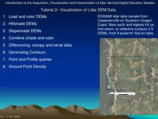
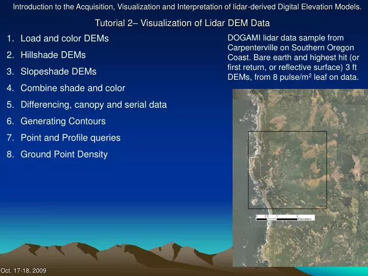
Load and color DEMs Hillshade DEMs Slopeshade DEMs Combine shade and color Differencing, canopy and serial data Generating Contours Point and Profile queries Ground Point Density.

E N D
Load and color DEMs • Hillshade DEMs • Slopeshade DEMs • Combine shade and color • Differencing, canopy and serial data • Generating Contours • Point and Profile queries • Ground Point Density DOGAMI lidar data sample from Carpenterville on Southern Oregon Coast. Bare earth and highest hit (or first return, or reflective surface) 3 ft DEMs, from 8 pulse/m2 leaf on data.
Load and color DEM • Add data> Bare_Earth_DEM and Highest_hit_DEM • Native scheme is grayscale with low values dark • Right click layer> properties> symbology • Select your preferred color scheme • Note differences between the two DEMs • DEM image alone is not a particularly useful visualization
Hillshade visualization • Arc Toolbox> 3D Analyst> Raster Surface> Hillshade • Input, Bare_Earth_DEM, set output to be_hs_315.img, accept defaults and run • Input Bare_Earth_DEM, set output to be_hs_225.img, set azimuth to 225 and run • Note difference in hillshades, some illumination angles simply don’t work. • Experiment with highest_hit_DEM, Azimuth, Altitude, Z factor, shadows
Slopeshade Visualization • Arc Toolbox> 3D analyst> Raster surface> slope • Input Bare_earth_DEM, set output to be_slope.img, run • Default color scheme is poison-dart frog • Right click layer> properties> symbology> choose stretched, invert, standard deviations and set n to 5 • Slopeshade map is “universal hillshade”. • Shading curve can be adjusted to illuminate features in the very steep or very gentle ends of the slope range, under Symbology, click histograms and play with nodes on curve to reshape • Experiment with Highest_hit_DEM
Combine layers • Turn off all layers • Load orthoimage • Right click layer> properties> display> set transparency to 50% • Turn on highest hit hillshade or slopeshade • Turn off all layers except beslope and Bare_Earth_DEM. Drag beslope below Bare_Earth_DEM, set Bare_Earth_DEM display to 50% transparency. This combination is very useful for mapping geologic and geomorphic features • Play with combinations of layers! • 70 % orthoimage over 70% highest hit hillshade over bare earth slopeshade makes a nice basemap.
Differencing;Canopy Height • Turn off all layers • Load Highest_Hit_DEM and Bare_Earth_DEM • Arc Toolbox> 3D Analyst> Raster Math> Minus • Use Highest_Hit_DEM for input 1, Bare_Earth_DEM for input 2, canopy.img for output, run • Right click canopy layer> properties> display> set transparency to 50% then symbology and choose your favorite color scheme • Turn on highest hit hillshade or slopeshade and position under canopy. • Combined image shows the height of vegetation, structures, can you find the transmission lines? • Note negative values in canopy. Highest hit and bare earth surfaces are made from different collections of points.
Differencing;Serial Data • Turn off all layers • Load be_leaf_off and be_leaf_on, select one and click zoom to layer • Arc Toolbox> 3D Analyst> Raster Math> Minus • Use be_leaf_off for input 1, be_leaf_on for input 2, serial.img for output, run • Right click serial layer> properties> display> set transparency to 50% then symbology> classified, say yes to create histogram, click on classify, and set values to -3, -1, 1 and 3. Click ok to return to main symbology tab, double click patches to select color, set lowest purple, next blue, next (-1 to 1) to “no color” next to orange, highest to red. • Load leaf_off_beslope and place it under serial • Image now shows areas of erosion as orange and red, deposition as blue and purple. You should be able to find two landslides and three debris flow scars. • Widespread noise is due to differences in ground models under heavy vegetation • Serial comparisons require high quality data.
Contours • Arc Toolbox> 3D Analyst> Raster Surface> Contour • Input be_leaf_off.img, accept default output, set contour interval to 1, run. • Resultant 1m contours provide additional detail on shape of landscape, particularly in areas of low slope. • Contours can greatly slow down redraw, minimize this by using contour with barriers and selecting a 1km grid file as the barrier. • Contours from lidar can be very rough, reflecting the high resolution of the DEM and the natural roughness of the surface. For nicer looking contours without significant loss of accuracy, use Arc Toolbox> Spatial Analyst> Neighborhood> Focal Statistics to smooth DEM before contouring.
Query Lidar, Point and profile • Turn off all layers • Turn on slope_be and canopy, select one and click zoom to layer • Click on info tool, select all visible layers, click on point of interest to see point location and elevation values • From main menu select View> Toolbars> and check 3D Analyst • In 3D Analyst toolbar, click layer list control and select canopy • From 3D Analyst toolbar select interpolate line, draw line across area of interest. • Initial interpolate line will be slow while grid is indexed. • When line appears, select create profile graph from 3D Analyst toolbar • Profile will appear in window, which can be stretched in X or Y. • Right click profile to see print and export options.
Ground Point Density • It is important to understand how good the data behind your DEM is, and ground point density is critical • Add the file 42124B3317.GPD, right click the layer and select zoom to layer • This is a vendor-supplied ground point density grid, white areas have > 1 ground point per 4m2, black areas less. • Zoom to a large area of black, and then turn off the GPD grid, leave on only the be_slope grid, note the obvious TIN triangle outlines in the grid. This is a simple graphic indicator of ground point density. Use the measurement tool to measure some of the TIN side lengths, some are quite long. • To make your own groundpoint density grid Arc Toolbox> Conversion> From File> LAS to Multipoint, choose 44124B3317_ground as input, ground_points as output, point spacing of 2 and run. • Select Arc Toolbox> Conversion Tools> To Raster > Point to Raster, use ground_points as input, pointcount as value field, accept default output, set cell assignment type to COUNT, cellsize to 15 and run. • Assign a color scheme to the resulting raster, make it 50% transparent and drape over the be_slope layer. Examine how the DEM looks in areas of low point density.
http://blogs.esri.com/Dev/blogs/geoprocessing/archive/2008/11/06/Lidar-Solutions-in-ArcGIS_5F00_part-1_3A00_-Assessing-Lidar-Coverage-and-Sample-Density.aspxhttp://blogs.esri.com/Dev/blogs/geoprocessing/archive/2008/11/06/Lidar-Solutions-in-ArcGIS_5F00_part-1_3A00_-Assessing-Lidar-Coverage-and-Sample-Density.aspx http://cws.unavco.org:8080/cws/learn/uscs/2008/2008Lidar/handouts/GeoEarthScopeDataTutorialApril08.pdf <http://cws.unavco.org:8080/cws/learn/uscs/2008/2008Lidar/handouts/GeoEarthScopeDataTutorialApril08.pdf> http://cws.unavco.org:8080/cws/learn/uscs/2008/2008Lidar/handouts/GLW_and_ArcMap.pdf <http://cws.unavco.org:8080/cws/learn/uscs/2008/2008Lidar/handouts/GLW_and_ArcMap.pdf> http://arrowsmith410-598.asu.edu/Lectures/Lecture14/ <http://arrowsmith410-598.asu.edu/Lectures/Lecture14/> http://arrowsmith410-598.asu.edu/Lectures/Lecture15/ <http://arrowsmith410-598.asu.edu/Lectures/Lecture15/> Additional Resources