Download
1 / 27
270 likes | 435 Views
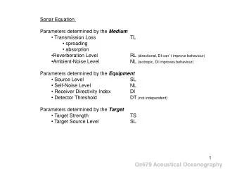
Sonar Equation Parameters determined by the Medium Transmission Loss TL spreading absorption Reverberation Level RL (directional, DI can ’ t improve behaviour) Ambient-Noise Level NL (isotropic, DI improves behaviour) Parameters determined by the Equipment Source Level SL

E N D
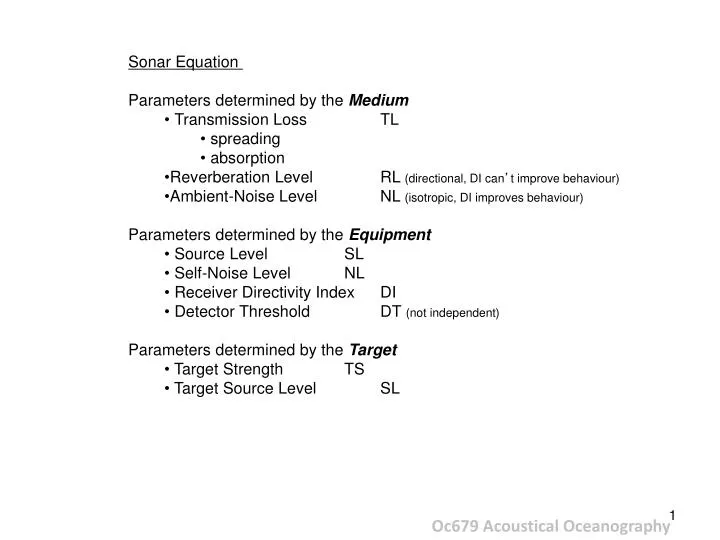
Sonar Equation • Parameters determined by the Medium • Transmission Loss TL • spreading • absorption • Reverberation Level RL (directional, DI can’t improve behaviour) • Ambient-Noise Level NL (isotropic, DI improves behaviour) • Parameters determined by the Equipment • Source Level SL • Self-Noise Level NL • Receiver Directivity Index DI • Detector Threshold DT (not independent) • Parameters determined by the Target • Target Strength TS • Target Source Level SL Oc679 Acoustical Oceanography
Units N = 10 log10 where I0 is a reference intensity the unit of N is deciBels so we might say that Iand I0 differ by N dB in terms of acoustic pressure, (p/p0)2 I/I0 where the oceanographic standard is p0 = 1 Pa in water we can write this in terms of pressure as 20 log10 • for comparison: • atmospheric pressure is 100 kPa • pressure increases at the rate of 10 kPa per meter of depth from the surface down • p/p0dB = 20log10p/p0 • 1 0 • √2 3 (double power level) • 2 6 • 4 12 • 10 20 • 20 26 • 100 40 • 1000 60 compare p/p0=1/√2, I/I0 = ½ dB = -3 we might say the -3dB level or ½ power level Oc679 Acoustical Oceanography
1 Pa is equivalent to 0 dB dB logarithmic scale linear scale
skeleton of array used on subs plane transducer array cylindrical transducer array Sources and Receivers pulsating sphere– an idealization to ease theoretical treatment - this is a monopole source in which the radiated sound is same amplitude and phase in all directions [ bubbles act as natural pulsating spheres ] sources and receivers (transducers) are actually designed with a wide range of properties physical, geometrical, acoustical and electrical proper design is necessary to provide appropriate sensitivity to specified frequencies or to specific propagation directions Oc679 Acoustical Oceanography
light bulb source / implosive source roughly 6 db force ~ the pressure difference across the glass Energy available ~ δp2 A doubling of depth (100m to 200 m) ought to result in a quadrupling of SL this corresponds to 6 dB for a doubling in depth
piezo – from Greek, “meaning to squeeze or press” piezoelectric – generates a voltage when piezo’d (& v.v) example: phonograph cartridge
CW source Pulsating Sphere – radial coordinates monopole instantaneous radial velocity at surface of pulsating sphere (radius a) is where Ua is the amplitude of the sphere’s radial velocity combining this with the expression for the isotropic radiated pressure at R and the particle velocity in radial coordinates gives an expression for the magnitude of the acoustic pressure at R [ this is written differently than in text ] • from this we can see that: • for constant Ua, the radiated acoustic pressure is proportional to the frequency of the CW source • for a given frequency (written as either or k) radiated acoustic pressure is proportional to the volume flow rate at the source (a2Ua) • for fixed kand a2Ua, the radiated sound pressure is proportional to acoustic impedance Ac Oc679 Acoustical Oceanography
dipole movie Dipole This can be considered as two equal strength monopoles that are out of phase and a small distance, d apart (such that kd<<1). There is no net introduction of fluid by a dipole. As one source exhales, the other source inhales and the fluid surrounding the dipole simply sloshes back and forth between the sources. It is the net force on the fluid which causes energy to be radiated in the form of sound waves. monopole movie Monopole longitudinal quadrupole movie Quadrupole This can be considered as four monopoles with two out of phase with the other two. They are either arranged in a line with alternating phase or at the vertices of a cube with opposite corners in phase. In the case of the quadrupole, there is no net flux of fluid and no net force on the fluid. It is the fluctuating stress on the fluid that generates the sound waves. However, since fluids don’t support shear stresses well, quadrupoles are poor radiators of sound. Longitudinal Quadrupole
Relative radiation efficiency of a quadrupole: Relative radiation efficiency of a dipole:
Sound Sources including sources, the wave equation can be written as 1 2 3 • where the 3 terms on the RHS are mechanical sources of radiated acoustic pressure • acceleration of mass per unit volume – this is associated with an injection (or removal) of mass at a point on a sound source [ as for example in a pulsating sphere or a siren (jet) which act as sources of new mass ] – this appears in the mass conservation equation which is later combined to get wave equation as it appears above • the divergence (spatial rate of change) of force (f) per unit volume – this is an adjustment to the conservation equation for momentum • associated with turbulence as an acoustic source – particularly important in explaining the noise caused by turbulence of a jet aircraft exhaust Oc679 Acoustical Oceanography
The Dipole 2 equal out-of-phase monopoles with a small separation (c.f. ) between them physically, it is straightforward to see that the 2 out-of-phase signals will completely cancel each other along a plane perpendicular to the line joining the 2 poles – they will partially cancel everywhere else far-field directionality is a figure 8 pattern in polar coordinates (cos in polar coordinates) idealized dipole dipole pressure expressed as 2 out-of-phase components for ranges large compared to separation l, use Fraunhofer approximation the small differences between R1 and R2 only important so far as defining phase differences (as kR1, kR2) – these are combined using the dipole condition ( kl << 1 ) to get the monopole pressure multiplied by iklcos 2 important results: - radiated pressure reduced by small factor kl c.f. monopole - radiation pattern no longer isotropic – directionality proportional to cos, where is the angle of the dipole axis – max along dipole line and 0 perpendicular to line Oc679 Acoustical Oceanography
dimensionless amplitude factor of nth source rate of attenuation due to absorption + scattering Line Arrays of Discrete Sources transducers typically constructed of multiple elements – some general tendencies can be discerned by consideration of a line of discrete sources equally separated over W separation between elements is pressure of nth source at range Rn and angle (that is, at Q): the far-field approximation allows us to replace Rn with R and we factor out the common terms leaving a factor that describes the transducers directional pressure response so Dt has magnitude and direction Oc679 Acoustical Oceanography
amplitude factors of the individual sources can be normalized such that • the choice of an determines the fundamental characteristics of the transducer • typically these choices are selected to • reduce side lobes • narrow central lobe • one choice (the simplest) is , • equal weighting to each transducer • other choices shown at right • this is basically a plot of transducer gain as a function of angle from the perpendicular to the line array • tendency: • for the same number of elements, weightings that decrease side lobes also widen main beam main beam boxcar side lobe side lobe triangle main beam side lobe cosine main beam Gaussian main beam no side lobe Oc679 Acoustical Oceanography
this can be extended to a continuous line source sinc function, sin(x)/x which is the Fourier transform of a boxcar beam pattern in polar coordinates far-field radiation from a boxcar line source this is the result of a 1D line source (i.e., point sources aligned along a single coordinate axis) suppose the sources aligned in 2D - this would result in a rectangular source whose directional response would be the product of the response in the 2 coordinate directions rectangular piston source – individual elements are closely-spaced, in phase and have the same amplitude Oc679 Acoustical Oceanography
Circular Piston Source far-field this would be similar to the kinds of transducers we see in echosounders, ADCPs as a piston source this has uniform, in phase amplitude across a circular cross-section so the directivity Dt is similar to a sinc function (but with a Bessel function involved) Dt in polar coordinates – beam pattern of circular piston transducer ka refers to the ratio of piston diameter to source wavelength a well-formed beam does not appear until ka becomes >> 1 we want the wavelength to be << physical dimension of the source transducer Oc679 Acoustical Oceanography
Circular Piston Source near-field complex pattern in near-field due to interference of radiation from different areas on the disk along disk axis, there is a critical range Rc beyond which interference is minimal ( that is, constructive interference cannot occur ) the range at which a receiver is safely in the far-field is arbitrary, since some interference will occur past the point where maximum destructive interference ceases this means that the definition of far-field in part depends on what level of S/N is required by the user this complexity means that it is impossible to measure P0 at 1 m from the source rather it must be measured in the far-field and extrapolated back to the source ( 1/R) this is how SL is determined for use in the sonar equation Oc679 Acoustical Oceanography
logarithmic polar plot ( ka = 20 ) there are several descriptors that incorporate beam strength, radiation pattern and directivity so that transducers can be compared quantitatively as you find when selecting electronic components, different manufacturers use different criteria - so you may need to do a little homework to understand what they mean – start with M&C sec 4.5.2 and other (better) transducer references but you may eventually have to talk to an engineer One criterion is the half-intensity beam width directional response of a circular piston transducer radius a half-intensity beam width defined at ½-power point: D2= 0.5 ( -3 db) interpretive example: consider 100 kHz source, a=10 cm k = 2f/c = 420 rad/m [ this means the acoustic wavelength is = 2/k= 0.015 m ] kasin = 1.6 when = 2.2 half intensity beam width = 2 = 4.4 Oc679 Acoustical Oceanography
property of the medium property of the wave SOURCE LEVEL – recall our solutions to the acoustic wave equation acoustic impedance satisfy plane waves of form substitution into [w1] integrating w.r.t. x note resemblance to Ohm’s law V = ZI where V is voltage, Z is impedance and I is current Ac, or rho-c is the acoustic impedance and is a property of the material
atmospheric pressure (105 Pa = 1011Pa) typical source level ?
what about displacement? = so the displacement required to produce a particular acoustic pressure, or a particular source level, is inversely proportional to frequency
Use of SONAR EQUATION to calibrate microstructure backscatter • acoustic backscatter strength • dashed line – direct measurement calibrated using sonar equation • solid line – model of microstructure backscatter [Bragg scattering from index of refraction fluctuations]
Example % calibrate – all units are dB RL=20*log10(bio.avsample); % receiver level (this is what we measure) SL=225; % source level (from calibration) RS=-39.25; % receiver sensitivity (from BioSonics cal) TL=20*log10(bio.depth-4.5)+0.045*(bio.depth-4.5); % 1-way transmission loss at range bio.depth) % solve for target strength [ RL=SL+RS-TL+TS ] this is an additive function that replaces the multiplicative system transfer function TS=-SL+RL-RS+2.*TL; TL= 29.3 dB at 35m range RL= 56 dB solve for: the 2 appears with TL here because the reflected signal is treated as a new source with the same range TS=RL-SL-RS+2.*TL = -70 dB Measured signal [V] / Sensitivity [V/Pa] this example taken from my code to calibrate BioSonics echosounder in units of dB Oc679 Acoustical Oceanography