Download
1 / 35
350 likes | 511 Views
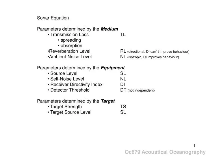
Sonar Equation Parameters determined by the Medium Transmission Loss TL spreading absorption Reverberation Level RL (directional, DI can ’ t improve behaviour) Ambient-Noise Level NL (isotropic, DI improves behaviour) Parameters determined by the Equipment Source Level SL

E N D
Sonar Equation • Parameters determined by the Medium • Transmission Loss TL • spreading • absorption • Reverberation Level RL (directional, DI can’t improve behaviour) • Ambient-Noise Level NL (isotropic, DI improves behaviour) • Parameters determined by the Equipment • Source Level SL • Self-Noise Level NL • Receiver Directivity Index DI • Detector Threshold DT (not independent) • Parameters determined by the Target • Target Strength TS • Target Source Level SL Oc679 Acoustical Oceanography
Units N = 10 log10 where I0 is a reference intensity the unit of N is deciBels so we might say that Iand I0 differ by N dB in terms of acoustic pressure, (p/p0)2 I/I0 where the oceanographic standard is p0 = 1 Pa in water we can write this in terms of pressure as 20 log10 • for comparison: • atmospheric pressure is 100 kPa • pressure increases at the rate of 10 kPa per meter of depth from the surface down • p/p0dB = 20log10p/p0 • 1 0 • √2 3 (double power level) • 2 6 • 4 12 • 10 20 • 20 26 • 100 40 • 1000 60 compare p/p0=1/√2, I/I0 = ½ dB = -3 we might say the -3dB level or ½ power level Oc679 Acoustical Oceanography
1 Pa is the reference standard for water 20 Pa is the reference standard for air 20 Pa 1 Pa 20log20 = 26 dB
small target (relative to λ) (Rayleigh scattering) large target (relative to λ) Scattering
Scattering scattering of light follows essentially the same scattering laws as sound but light wavelengths are much smaller than sound - O(100s of nm) almost all scattering bodies in seawater are large compared to optical wavelengths and have optical cross-sections equal to their geometrical cross-sections Large Targets the sea is turbid to light on the other hand, acoustic wavelengths are typically large compared to scattering bodies found in seawater (at 300 kHz, 5 mm, 4 orders of magnitude larger) - acoustic scattering is dominated by Rayleigh scattering Small Targets by comparison the sea is transparent to sound - what limits the propagation of 300 kHz sound is not scattering but absorption
TL • Absorption • in a homogeneous medium, a plane wave experiences an attenuation of acoustic pressure the original pressure and to the distance traveled – this is represented by a bulk viscosity in the N-S equations which applies only to compressible fluid (this is distinct from a shear viscosity – M&C sec 3.4.2) • this is due To wave absorption (energy lost to heat) • e is the amplitude decay coefficient • absorption losses are due to ionic dissociation that is alternately activated and deactivated by sound condensation and rarefaction • the attenuation by this manner in SW is 30x that in FW • dominated by magnesium sulphate and boric acid acoustic absorption absorption typical profiling frequency @S=0 @S=35 range 3000 kHz 2.4 dB/m 2.5 dB/m 3-6 m 1500 kHz 0.60 dB/m 0.67 dB/m 15-25 m 500 kHz 0.07 dB/m 0.14 dB/m 70-110 m source: Sontek ADCP manual Oc679 Acoustical Oceanography
TL relate spherical spreading & range attenuation due to absorption in terms of sonar equation spherical spreading 1/R2, that is log10 I/I0 = log10R02/R2= log10R02 – log10R2 but since typically I0is referred to 1 m range from source, log10R02=0 and 10log10I/I0 = – 20log10R range attenuation related by p = p0e-R, or I = I0e-2R then 10log10I/I0 = - 20R and together these represent a transmission loss TL = -20log10R - 20R absorption spherical spreading Oc679 Acoustical Oceanography
TL cylindrical spreading is an approximation to propagation through sound channel analogue is propagation through medium with plane-parallel upper and lower bounds this is important for long range transmission through sound channel – since the loss is now 1/R rather than 1/R2, propagation is more efficient this doesn’t happen Spreading Oc679 Acoustical Oceanography
TL Spherical component Spreading • Spreading • Due to divergence • No loss of energy • Sound spread over wide area • Two types: • Spherical • Short Range: R < 1000m • TL (dB) = 20 log R • Cylindrical • Long Range: R > 1000m • TL (dB) = 10 log R + 30 dB
now consider the reflected signal from a target with reflection coefficient R12 p is the pressure at range R R12 is the target reflection coefficient Srec is the receiver sensitivity [ Pa/V ] V is the voltage o/p measured at receiver 0 RS RL SL TL TS this is the voltage measured at the receiver – more commonly this would be in counts, which is then converted to volts Oc679 Acoustical Oceanography
this is the physical relationship that we have developed this is how that relationship is represented logarithmically terms in the SONAR EQUATION represent logarithms
let’s take a step back now that we have seen how the SONAR EQUATION is formed the physics is straightforward as is the transformation to a logarithmic equations – more straightforward than is implied by the large number of variations to the SONAR EQUATION that appear – these are usually specific to the application and intended for unambiguous use by operators we’ll look at a couple of variations
Passive SONAR EQUATION passive sonars listen only purpose – detection, classification and localization of an acoustic source in turn, a particular source is embedded in a sea of sources suppose a radiating object of source level SL (decibels) is received at a hydrophone at a lower signal level S due to transmission loss TL (TL always > 0) S = SL – TL where we have already defined TL = 20log10R + 20R to be due to the product of absorption and spreading (which appear additively in this logarithmic representation) and we could represent the signal to noise ratio at the hydrophone as SNR = SL – TL – N logarithmic representation of this is the logarithmic representation of
DI directivity index SNR can be increased by beam-forming so that sound does not spread spherically but is more directional for an omnidirectional source I is proportional to 4πR2 here it is constrained to πr2 where r might be the piston diameter of a cylindrical source Define DI = 10log(intensity of acoustic beam /intensity of omnidirectional source) DI = 10 log ((p/πr2)/(p/4πR2)) r r S R = 1 m α/2 with R = 1 DI = 10 log (4/r2) and tan(α) = r/R = r DI = 10 log (4/tan2(α/2))
SNR can be increased by beam-forming produced by an array of transducers (perhaps in a single head or maybe distributed geographically) the directivity index DI represents this advantage for a particular array so that SNR = SL – TL – N + DI ideally, detection is possible when the signal is sufficiently close and not disguised by noise … that is, when SNR > 0 however, due to the nature of the signal, interference, the sonar operator’s training and alertness, etc … something more than 0 is necessary this extra appears as a detection threshold, DT we now write the SONAR EQUATION in terms of a signal excess SE SE = SL – TL – N + DI – DT this is now the difference between the actual received signal at the output of the beamformed array and minimum signal required for detection
if DT set to be too high, only targets with high source levels are detected. Detection may be difficult but the probability of a false alarm is low as well. On the other hand, if DT is too low, the probability of false alarms increases
Looking at a single trace on an oscilloscope is a little antiquated. A time history helps to see what’s going on.
Active SONAR EQUATION now the transducer transmits a signal that is reflected or scattered from an object – the modified signal is sensed at the receiver (which may be the same as the source, in monostatic mode) this modified signal must be extracted from the background interference which is not only the sonar noise and ambient noise, but also the reverberation generated by the original signal simple example – travel-time measurement of the echo to estimate the distance to an object (such as a fathometer which measures water depth by listening to the echo of a ping off the sea floor) we can simply say that the sound pressure level SPL at range R is SPL = SL - TL
three principal differences from passive case • received signal level modified by target strength TS • reverberation is the dominant interference • transmission loss results from 2 paths • transmitter to target + target to receiver • monostatic - transmission loss is 2TL • bistatic - transmission loss is TL1 + TL2 • Reverberation Level RL • results primarily from scattering of the transmitted • signal from things other than the target of interest • boundary scattering may be due to waves, ice bottom features • volume scattering may be due to zooplankton, fish, microstructure, … • this means that the total interference term is due to the sum of the noise and the reverberation N + RL – these act to diminish our ability to detect TS
Homework 1 – Martin Hoecker-Martinez 18 Jan 2011 http://wart.coas.oregonstate.edu/Documents/for%20others/jim/150W.gif
So, there are essentially two types of background that may mask the signal that we wish to detect: • Noise background or Noise Level (NL). This is an essentially a steady state, isotropic (equal in all directions) sound which is generated by amongst other things wind, waves, biological activity and shipping. This is in addition to transducer system self-noise. (Wenz curves) • 2) Reverberation background or reverberation level (RL). This is the slowly decaying portion of the back-scattered sound from one's own acoustic input. Excellent reflectors in the form of the sea surface and floor bound the ocean. Additionally, sound may be scattered by particulate matter (e.g. plankton) within the water column. You will have experienced reverberation for yourself. For example if you shout loudly in a cave you are likely to here a series of echoes reverberating due to sound reflections from the hard rock surfaces. These reverberations decay rapidly with time. • Although both types of background are generally present simultaneously it is common for either one or the other to be dominant.
we could define SONAR EQUATION for a monostatic system as SE = SL – 2TL + TS – (RL + N) + DI – DT And for a bistatic system SE = SL – TL1 + TS – TL2 – (RL + N) + DI – DT
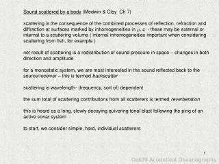
Sound scattered by a body - RL in SONAR EQUATION scattering is the consequence of the combined processes of reflection, refraction and diffraction at surfaces marked by inhomogeneities in c - these may be external or internal to a scattering volume ( internal inhomogeneities important when considering scattering from fish, for example ) net result of scattering is a redistribution of sound pressure in space – changes in both direction and amplitude the sum total of scattering contributions from all scatterers is termed reverberation this is heard as a long, slowly decaying quivering tonal blast following the ping of an active sonar system consideration usually begins by considering scattering from spheres Oc679 Acoustical Oceanography
direct signal explosive source at 250 m nearby receiver at 40 m bottom depth 2000 m reverberation following explosive charge initial surface reverb is sharp, followed by tail due to multiple reflection & scattering then volume reverb in mid-water column (incl. deep scattering layer) then bottom reflection, 2nd surface reflection, and long tail of bottom reverb Oc679 Acoustical Oceanography
sounds in the sea or N in the SONAR EQUATION natural physical sounds natural biological sounds ships Oc679 Acoustical Oceanography
Wenz curves used to determine ambient noise thick black line – empirical minimum A - seismic noise B – ship noise (shallow water) C – ship noise (deep water) H – hail W – sea surface sound at 5 wind speeds R1 – drizzle (1 mm/h) 0.6 m/s wind over lake R2 – drizzle, 2.6 m/s wind over lake R3 – heavy rain (15 mm/h) at sea R4 – v. heavy rain (100 mm/h) at sea F – thermal noise (f1) - molecular Oc679 Acoustical Oceanography
on-axis source level spectra of cargo ship at 8 & 16 kts measured directly below ship – this represents the details of what we saw in the compilation slides B – propeller Blade rate F – diesel engine Firing rate G – ship’s service Generator rate Oc679 Acoustical Oceanography
propagation of coastal shipping noise into deep sound channel c(z) this is due to c(z) profile over the shelf, causing a progression of sound down the slope until the axis of the deep sound channel is reached after that, a reversal of refraction occurs, and signal trapped in sound channel coastal shipping noise can be propagated long distances Oc679 Acoustical Oceanography
Homework Assignment 2 assigned: 18 Jan 2010 due: 27 Jan 2010 A yellow submarine is conducting a passive search against blue submarines. Yellow submarines have a sonar with directivity index of 15 dB and detection threshold 8 dB. Blue submarines have known source level 140 dB. Environmental conditions yield an isotropic noise level of 65 dB. You can assume an absorption decay coefficient 0.02 dB/km. At what range can the blue submarine be detected by the yellow submarine? Show your answer graphically.