The Big Picture: Where are We Now?

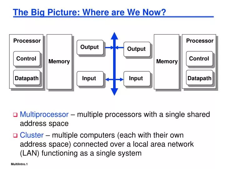
1. The Big Picture: Where are We Now? • Multiprocessor – multiple processors with a single shared address space • Cluster – multiple computers (each with their own address space) connected over a local area network (LAN) functioning as a single system Processor Processor Output Output Control Control Memory Memory Datapath Input Input Datapath

2. Applications Needing “Supercomputing” • Energy (plasma physics (simulating fusion reactions), geophysical (petroleum) exploration) • DoE stockpile stewardship (to ensure the safety and reliability of the nation’s stockpile of nuclear weapons) • Earth and climate (climate and weather prediction, earthquake, tsunami prediction and mitigation of risks) • Transportation (improving vehicles’ airflow dynamics, fuel consumption, crashworthiness, noise reduction) • Bioinformatics and computational biology (genomics, protein folding, designer drugs) • Societal health and safety (pollution reduction, disaster planning, terrorist action detection)

3. Exec time w/o E Speedup w/ E = ---------------------- Exec time w/ E Encountering Amdahl’s Law • Speedup due to enhancement E is • Suppose that enhancement E accelerates a fraction F (F <1) of the task by a factor S (S>1) and the remainder of the task is unaffected ExTime w/ E = ExTime w/o E  ((1-F) + F/S) Speedup w/ E = 1 / ((1-F) + F/S)

4. Examples: Amdahl’s Law Speedup w/ E = 1 / ((1-F) + F/S) • Consider an enhancement which runs 20 times faster but which is only usable 25% of the time. Speedup w/ E = 1/(.75 + .25/20) = 1.31 • What if its usable only 15% of the time? Speedup w/ E = 1/(.85 + .15/20) = 1.17 • Amdahl’s Law tells us that to achieve linear speedup with 100 processors, none of the original computation can be scalar! • To get a speedup of 99 from 100 processors, the percentage of the original program that could be scalar would have to be 0.01% or less

5. Supercomputer Style Migration (Top500) http://www.top500.org/lists/2005/11/ • In the last 8 years uniprocessor and SIMDs disappeared while Clusters and Constellations grew from 3% to 80% Nov data Cluster – whole computers interconnected using their I/O bus Constellation – a cluster that uses an SMP multiprocessor as the building block

6. Multiprocessor/Clusters Key Questions • Q1 – How do they share data? • Q2 – How do they coordinate? • Q3 – How scalable is the architecture? How many processors can be supported?

7. Flynn’s Classification Scheme • SISD – single instruction, single data stream • aka uniprocessor - what we have been talking about all semester • SIMD – single instruction, multiple data streams • single control unit broadcasting operations to multiple datapaths • MISD – multiple instruction, single data • no such machine (although some people put vector machines in this category) • MIMD – multiple instructions, multiple data streams • aka multiprocessors (SMPs, MPPs, clusters, NOWs)

8. PE PE PE PE PE PE PE PE Control PE PE PE PE PE PE PE PE SIMD Processors • Single control unit • Multiple datapaths (processing elements – PEs) running in parallel • Q1 – PEs are interconnected (usually via a mesh or torus) and exchange/share data as directed by the control unit • Q2 – Each PE performs the same operation on its own local data

9. Example SIMD Machines

10. Multiprocessor Basic Organizations • Processors connected by a single bus • Processors connected by a network

11. Shared Address (Shared Memory) Multi’s • Q1 – Single address space shared by all the processors • Q2 – Processors coordinate/communicate through shared variables in memory (via loads and stores) • Use of shared data must be coordinated via synchronization primitives (locks) • UMAs (uniform memory access) – aka SMP (symmetric multiprocessors) • all accesses to main memory take the same amount of time no matter which processor makes the request or which location is requested • NUMAs (nonuniform memory access) • some main memory accesses are faster than others depending on the processor making the request and which location is requested • can scale to larger sizes than UMAs so are potentially higher performance

12. N/UMA Remote Memory Access Times (RMAT)

13. Single Bus (Shared Address UMA) Multi’s • Caches are used to reduce latency and to lower bus traffic • Must provide hardware to ensure that caches and memory are consistent (cache coherency • Must provide a hardware mechanism to support process synchronization Processor Processor Processor Cache Cache Cache Single Bus Memory I/O

14. Summing 100,000 Numbers on 100 Processors • Processors start by running a loop that sums their subset of vector A numbers (vectors A and sum are shared variables, Pn is the processor’s number, i is a private variable) sum[Pn] = 0; for (i = 1000*Pn; i< 1000*(Pn+1); i = i + 1) sum[Pn] = sum[Pn] + A[i]; • The processors then coordinate in adding together the partial sums (half is a private variable initialized to 100 (the number of processors)) repeat synch(); /*synchronize first if (half%2 != 0 && Pn == 0) sum[0] = sum[0] + sum[half-1]; half = half/2 if (Pn<half) sum[Pn] = sum[Pn] + sum[Pn+half] until (half == 1); /*final sum in sum[0]

15. sum[P0] sum[P1] sum[P2] sum[P3] sum[P4] sum[P5] sum[P6] sum[P7] sum[P8] sum[P9] P0 P1 P2 P3 P4 P5 P6 P7 P8 P9 P0 P1 P2 P3 P4 P0 P1 P0 An Example with 10 Processors half = 10 half = 5 half = 2 half = 1

16. Message Passing Multiprocessors • Each processor has its own private address space • Q1 – Processors share data by explicitly sending and receiving information (messages) • Q2 – Coordination is built into message passing primitives (send and receive)

17. Summary • Flynn’s classification of processors – SISD, SIMD, MIMD • Q1 – How do processors share data? • Q2 – How do processors coordinate their activity? • Q3 – How scalable is the architecture (what is the maximum number of processors)? • Shared address multis – UMAs and NUMAs • Bus connected (shared address UMAs) multis • Cache coherency hardware to ensure data consistency • Synchronization primitives for synchronization • Bus traffic limits scalability of architecture (< ~ 36 processors) • Message passing multis