Download
1 / 83
900 likes | 1.24k Views
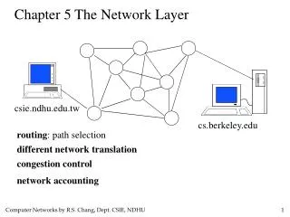
Chapter 5 The Network Layer. review. How many layers have the OSI’s model divided the network architecture into?. Seven layers. APPLICATION. PRESENTATION. What are they from the bottom to the top?. SESSION. TRANSPORT. NETWORK. ISO/OSI’s network model. DATA LINK. PHYSICAL.

E N D
review How many layers have the OSI’s model divided the network architecture into? Seven layers APPLICATION PRESENTATION What are they from the bottom to the top? SESSION TRANSPORT NETWORK ISO/OSI’s network model DATA LINK PHYSICAL
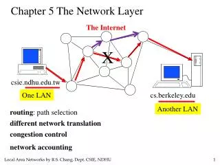
Description of the network layer • To achieve its goals, the network layer must know about the topology of the communica-tion subnet and choose appropriate paths th-rough it. It must also take care to choose routes to avoid overloading some of the commun-ication lines and routers while leaving others idle. • The network layer is concerned with getting packets from the source all the way to the destination.
Chapter 5 The Network Layer 5.1 Network Layer Design Issues 5.2 Routing Algorithms 5.6 The Network Layer in the Internet
5.1 Network Layer Design Issues • Store-and-Forward Packet Switching • Services Provided to the Transport Layer • Implementation of Connectionless Service • Implementation of Connection-Oriented Service • Comparison of Virtual-Circuit and Datagram Subnets
Store-and-Forward Packet Switching Customer’s equipment fig 5-1 The environment of the network layer protocols. • This equipment is used as follows:
A host with a packet to send transmits it to the nearest router, either on its own LAN or over a point-to-point link to the carrier. • The packet is stored there until it has fully arrived so the checksum can be verified. Then it is forwarded to the next router along the path until it reaches the destination host, where it is delivered. This mechanism is store-and-forward packet switching.
5.1 Network Layer Design Issues • Store-and-Forward Packet Switching • Services Provided to the Transport Layer • Implementation of Connectionless Service • Implementation of Connection-Oriented Service • Comparison of Virtual-Circuit and Datagram Subnets
Services Provided to the Transport Layer • The network layer services have been designed with the following goals: 1. The services should be independent of the router tech- nology. 2. The transport layer should be shielded from the num- ber, type, and topology of the routers present. 3. The network addresses made available to the transport layer should use a uniform numbering plan, even across LANs and WANs. What kind of services the network layer provides to the transport layer ?
One camp’s view The Internet offers connectionless network-layer service. The routers' job is moving packets around and no-thing else. In their view , the subnet is inherently un-reliable, no matter how it is designed. Therefore, the hosts should accept the fact that the network is unre-liable and do error control (i.e., error detection and correction) and flow control themselves. So the network service should be connectionless.
The other camp’s view ATM networks offer connection-oriented network-layer service. The subnet should provide a reliable, connection-oriented service. In this view, quality of service is the dominant factor, and without connections in the sub-net, quality of service is very difficult to achieve, esp-ecially for real-time traffic such as voice and video.
5.1 Network Layer Design Issues • Store-and-Forward Packet Switching • Services Provided to the Transport Layer • Implementation of Connectionless Service • Implementation of Connection-Oriented Service • Comparison of Virtual-Circuit and Datagram Subnets
Two different organizations are possible, depending on the type of service offered. • If connectionless service is offered, packets are injected into the subnet individually and routed independently of each other. No advance setup is needed. In this context, the packets are frequently called datagrams and the subnet is called a datagram subnet. • If connection-oriented service is used, a path from the source router to the destination router must be established before any data packets can be sent. This connection is called a VC (virtual circuit) and the subnet is called a virtual-circuit subnet.
Implementation of Connectionless Service P346 The question is: a packet with a destination D arrives at router A. then which router will router A send this packet to? Routing within a diagram subnet.
5.1 Network Layer Design Issues • Store-and-Forward Packet Switching • Services Provided to the Transport Layer • Implementation of Connectionless Service • Implementation of Connection-Oriented Service • Comparison of Virtual-Circuit and Datagram Subnets
For connection-oriented service, we need a virtual-circuit subnet. • The idea behind virtual circuits is to avoid having to choose a new route for every packet sent. Instead,when a connection is established, a route from the source machine to the destination machine is chosen as part of the connection setup and stored in tables inside the routers. That route is used for all traffic flowing over the connection, exactly the same way that the teleph-one system works. When the connection is released, the virtual circuit is also terminated. • With connection-oriented service, each packet carries an identifier telling which virtual circuit it belongs to.
Implementation of Connection-Oriented Service P347 Routing within a virtual-circuit subnet.
5.1 Network Layer Design Issues • Store-and-Forward Packet Switching • Services Provided to the Transport Layer • Implementation of Connectionless Service • Implementation of Connection-Oriented Service • Comparison of Virtual-Circuit and Datagram Subnets
Inside the subnet, several trade-offs exist between virtual circuits and datagrams. • One trade-off is between router memory space and bandwidth. • Virtual circuits allow packets to contain circuit numbers instead of full destination addresses. If the packets tend to be fairly short, a full destination address in every packet may represent a significant amount of overhead and hence, wasted bandwidth. • The price paid for using virtual circuits internally is the table space within the routers. Depending upon the relative cost of communication circuits versus router memory, one or the other may be cheaper.
Another trade-off is setup time versus address parsing time. • Using virtual circuits requires a setup phase, which takes time and consumes resources. However, figuring out what to do with a data packet in a virtual-circuit subnet is easy: the router just uses the circuit number to index into a table to find out where the packet goes. • In a datagram subnet, a more complicated lookup procedure is required to locate the entry for the destination.
Virtual circuits have some advantages in guaranteeing quality of service and avoiding congestion within the subnet. • The loss of a communication line is fatal to virtual circuits using it but can be easily compensated for if datagrams are used. Datagrams also allow the routers to balance the traffic throughout the subnet, since routes can be changed partway through a long sequence of packet transmissions.
Summary • 5.1 Network Layer Design Issues • Store-and-Forward Packet Switching • Services Provided to the Transport Layer • Implementation of Connectionless Service • Implementation of Connection-Oriented Service • Comparison of Virtual-Circuit and Datagram Subnets
Chapter 5 The Network Layer 5.1 Network Layer Design Issues 5.2 Routing Algorithms 5.6 The Network Layer in the Internet
Description of Routing Algorithms packet 1 Definition: The routing algorithm is that part of the network layer software responsible for deciding which output line an incoming packet should be transmitted on. 2 Properties of routing algorithm: correctness, simplicity, robustness, stability, fairness, and optimality.
Description of Routing Algorithms 1)Robustness: • Once a major network comes on the air, it may be expected to run continuously for years without system-wide failures. During that period there will be hardware and software failures of all kinds. Hosts, routers, and lines will fail repeatedly, and the topology will change many times. • The routing algorithm should be able to cope with changes in the topology and traffic without requiring all jobs in all hosts to be aborted and the network to be rebooted every time some router crashes.
Description of Routing Algorithms P A B Q equilibrium converge 2) Stability: It is also an important goal for the routing algorithm. There exist routing algorithms that never converge to equilibrium, no matter how long they run. A stable algorithm reaches equilibrium and stays there.
3) Fairness and optimality may sound obvious, but as it turns out, they are often contradictory goals. • There is enough traffic between A and A', between B and B', and between C and C' to saturate the horizontal links. To maximize the total flow, the X to X' traffic should be shut off altogether. Unfortunately, X and X' may not see it that way. Evidently, some compromise between global efficiency and fairness to individual connections is needed.
Description of Routing Algorithms B D A C D nonadaptive and adaptive 3 Category of algorithm: nonadaptive and adaptive. • Nonadaptive algorithms do not base their routing decisions on measurements or estimates of the current traffic and topology. Instead, the choice of the route to use to get from I to J is computed in advance, off-line, and downloaded to the routers when the network is booted. • This procedure is sometimes called static routing.
Description of Routing Algorithms B D A C D 2) Adaptive algorithms, in contrast, change their routing decisions to reflect changes in the topology, and usually the traffic as well. • This procedure is sometimes called dynamic routing.
5.2 Routing Algorithms • The Optimality Principle • Shortest Path Routing • Flooding • Distance Vector Routing • Link State Routing • Hierarchical Routing • Broadcast Routing
5.2.1 The Optimality Principle I K J • The Optimality Principle:if router J is on the optimal path from router I to router K, then the optimal path from J to K also falls along the same route.
5.2.1 The Optimality Principle • The set of optimal routes from all sources to a given destination form a tree rooted at the destination. Such a tree is called a sink tree. • Figure (a) A subnet. (b) A sink tree for router B.
5.2.1 The Optimality Principle • Note: A sink tree is not necessarily unique; other trees with the same path lengths may exist. • The goal of all routing algorithms is to discover and use the sink trees for all routers.
5.2.2 Shortest Path Routing • A technique to study routing algorithms: The idea is to build a graph of the subnet, with each node of the graph representing a router and each arc of the graph representing a communication line (often called a link). • To choose a route between a given pair of routers, the algorithm just finds the shortest path between them on the graph. • One way of measuring path length is the number of hops. Another metric is the geographic distance in kilometers . Many other metrics are also possible. For example, each arc could be labeled with the mean queuing and transmission delay for some standard test packet as determined by hourly test runs. • In the general case, the labels on the arcs could be computed as a function of the distance, bandwidth, average traffic, communication cost, mean queue length, measured delay, and other factors. By changing the weighting function, the algorithm would then compute the ''shortest'' path measured according to any one of a number of criteria or to a combination of criteria.
5.2.2 Shortest Path Routing (1930年5月11日~2002年8月6日) Dijkstra algorithm: • Each node is labeled (in parentheses) with its distance from the source node along the best known path. Initially, no paths are known, so all nodes are labeled with infinity. • As the algorithm proceeds and paths are found, the labels may change, reflecting better paths. • A label may be either tentativeor permanent. Initially, all labels are tentative. When it is discovered that a label represents the shortest possible path from the source to that node, it is made permanent and never changed thereafter.
P353 Next steps? • Figure. The first five steps used in computing the shortest path from A to D. The arrows indicate the working node. The shortest path from A to D is: ABEFHD
5.2.3 Flooding • Flooding algorithm:every incoming packet is sent out on every outgoing line except the one it arrived on. • Flooding obviously generates vast numbers of duplicate packets, in fact, an infinite number unless some measures are taken to damp the process. • One such measure is to have a hop counter contained in the header of each packet, which is decremented at each hop, with the packet being discarded when the counter reaches zero. • An alternative technique for damming the flood is to keep track of which packets have been flooded, to avoid sending them out a second time. • How to implement that? (P355)
5.2.3 Flooding • A variation of flooding that is slightly more practical is selective flooding.In this algorithm the routers do not send every incoming packet out on every line, only on those lines that are going approximately in the right direction. • Applications of flooding algorithm: • military applications • distributed database applications • wireless networks • as a metric against which other routing algorithms can be compared
5.2.4 Distance Vector Routing Lester Randolph Ford NO PHOTO Delbert Ray Fulkerson NO PHOTO August 26, 1920~March 19, 1984 • A dynamic routing algorithm • Distance vector routing algorithms operate by having each router maintain a table (i.e, a vector) giving the best known distance to each destination and which line to use to get there. These tables are updated by exchanging information with the neighbors. (also named the distributed Bellman-Ford routing algorithm and the Ford-Fulkerson algorithm ) September 23,1927~ August 14, 1924~January 10, 1976
5.2.4 Distance Vector Routing • Table content: In distance vector routing, each router maintains a routing table indexed by, and containing one entry for, each router in the subnet. This entry contains two parts: the preferred outgoing line to use for that destination and an estimate of the time or distance to that destination. • Table updating method: • Assume that the router knows the delay to each of its neighbors. Once every T msec each router sends to each neighbor a list of its estimated delays to each destination. It also receives a similar list from each neighbor. • Imagine that one of these tables has just come in from neighbor X, with Xi being X's estimate of how long it takes to get to router i. If the router knows that the delay to X is m msec, it also knows that it can reach router i via X in Xi + m msec. • By performing this calculation for each neighbor, a router can find out which estimate seems the best and use that estimate and the corresponding line in its new routing table. Note that the old routing table is not used in the calculation.
yyy • Part (a) shows a subnet. The first four columns of part (b) show the delay vectors received from the neighbors of router J. Suppose that J has measured or estimated its delay to its neighbors, A, I, H, and K as 8, 10, 12, and 6 msec, respectively.
5.2.5 Link State Routing • A dynamic routing algorithm • The idea behind link state routing can be stated as five parts. Each router must do the following: 1.Discover its neighbors and learn their network addresses. 2.Measure the delay or cost to each of its neighbors. 3.Construct a packet telling all it has just learned. 4.Send this packet to all other routers. 5.Compute the shortest path to every other router. • In effect, the complete topology and all delays are experimentally measured and distributed to every router. Then Dijkstra's algorithm can be run to find the shortest path to every other router.
5.2.5 Link State Routing 1. Learning about the Neighbors • It accomplishes this goal by sending a special HELLO packet on each point-to-point line. The router on the other end is expected to send back a reply telling who it is. • These names must be globally unique because when a distant router later hears that three routers are all connected to F, it is essential that it can determine whether all three mean the same F. 2. Measuring Line Cost • The most direct way to determine this delay is to send over the line a special ECHO packet that the other side is required to send back immediately. • By measuring the round-trip time and dividing it by two, the sending router can get a reasonable estimate of the delay. • For even better results, the test can be conducted several times, and the average used. Of course, this method implicitly assumes the delays are symmetric, which may not always be the case.
5.2.5 Link State Routing 3. Building Link State Packets • The packet starts with the identity of the sender, followed by a sequence number and age (to be described later), and a list of neighbors. For each neighbor, the delay to that neighbor is given. (a) A subnet. (b) The link state packets for this subnet
5.2.5 Link State Routing • Building the link state packets is easy. The hard part is determining when to build them. • One possibility is to build them periodically, that is, at regular intervals. • Another possibility is to build them when some significant event occurs, such as a line or neighbor going down or coming back up again or changing its properties appreciably. 4. Distributing the Link State Packets • The basic distribution algorithm:The fundamental idea is to use flooding to distribute the link state packets. • To keep the flood in check, each packet contains a sequence number that is incremented for each new packet sent. Routers keep track of all the (source router, sequence) pairs they see. • When a new link state packet comes in, it is checked against the list of packets already seen. • If it is new, it is forwarded on all lines except the one it arrived on. • If it is a duplicate, it is discarded. • If a packet with a sequence number lower than the highest one seen so far ever arrives, it is rejected as being obsolete since the router has more recent data.
5.2.5 Link State Routing • First problem with this algorithm:if the sequence numbers wrap around, confusion will reign. The solution here is to use a 32-bit sequence number. With one link state packet per second, it would take 137 years to wrap around, so this possibility can be ignored. • Second problem :if a router ever crashes, it will lose track of its sequence number. If it starts again at 0, the next packet will be rejected as a duplicate. • Third problem :if a sequence number is ever corrupted and 65,540 is received instead of 4 (a 1-bit error), packets 5 through 65,540 will be rejected as obsolete, since the current sequence number is thought to be 65,540.
5.2.5 Link State Routing • The solution to all these problems is to include the age of each packet after the sequence number and decrement it once per second. When the age hits zero, the information from that router is discarded. 5. Computing the New Routes • Once a router has accumulated a full set of link state packets, it can construct the entire subnet graph because every link is represented. • Now Dijkstra's algorithm can be run locally to construct the shortest path to all possible destinations.
5.2.6 Hierarchical Routing • The routers are divided into what we will call regions, with each router knowing all the details about how to route packets to destinations within its own region, but knowing nothing about the internal structure of other regions. • For huge networks, a two-level hierarchy may be insufficient; it may be necessary to group the regions into clusters, the clusters into zones, the zones into groups, and so on, until we run out of names for aggregations.
5.2.6 Hierarchical Routing zone cluster region cluster region zone region region region cluster region region region region region region cluster region