Download
1 / 43
430 likes | 627 Views
Training Schedule June 21, 2007 (afternoon). 02:00-03:30 UDEC Operation - System requirements, installation structure, manual volumes, files, nomenclature, system of units Model Generation* : [Build] tool Material Models* : [Blocks] tool

E N D
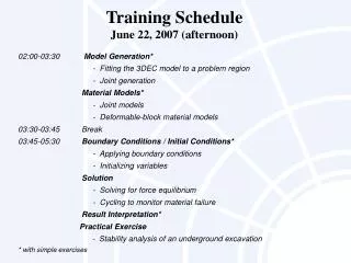
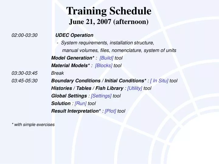
Training ScheduleJune 21, 2007 (afternoon) 02:00-03:30 UDEC Operation - System requirements, installation structure, manual volumes, files, nomenclature, system of units Model Generation* : [Build] tool Material Models* : [Blocks] tool 03:30-03:45 Break 03:45-05:30 Boundary Conditions / Initial Conditions* : [ In Situ] tool Histories / Tables / Fish Library : [Utility] tool Global Settings : [Settings] tool Solution : [Run] tool Result Interpretation* : [Plot] tool * with simple exercises
Getting Started • Starting UDEC • Memory Requirements • How to add RAM • Typical size of files
UDEC Files Project File (*.prj) - GUI project file Save File (*.sav) – Binary file containing values of all state variables and user-defined conditions at stage that file is saved Data File (*.dat) – ASCII file listing UDEC commands that represent the problem being analyzed History File (*.his) – ASCII file record of input or output history values Plot File – Graphics plot file (in various standard formats) Movie File (*.dcx) – String of PCX images that can be viewed as a “movie” Property File (*.gmt) – GUI property files (user may modify)
Nomenclature model outer boundary joint In situ horizontal boundary stress fault block cable earthquake ground motion structural lining interior boundary (excavation) zone gridpoint
Nomenclature • UDEC MODEL The model is created by a sequence of UDEC commands which define the problem conditions for numerical solution. • BLOCK: Fundamental geometric entity for the distinct element calculation. The UDEC model is created by “cutting” a single block into many smaller blocks. A block may be detached from or interact with other blocks through surface forces. • CONTACT Blocks are connected to each other through point contacts. Contact are boundary condition through which external forces to apply each block. • DISCONTINUITY A discontinuity is a geologic feature that separates a physical mass into distinct parts. Discontinuities are joints, faults, fractures and other discontinuities in a rock mass.
Nomenclature • DOMAIN The void or space between blocks. Domains are physical entities in the UDEC model; each domain is an enclosed region defined by two or more contacts. The “outer domain” is the region surrounding the model. Note that a domain exists between the adjoining faces of two overlapping blocks, even though the domain area appears to be negative. Contact detection is performed within domains. Fluid flow occurs between domains. • ZONE Deformable blocks are composed of finite-volume zones. Stress/strain and heat transfer are calculated within each zone. • GRIDPOINT Gridpoints are the corners of the zones. Each zone has 3 gridpoints. Each gridpoint has an x- and a y-coordinate. Gridpoints are sometime called nodes.
Nomenclature • MODEL BOUNDARY The periphery of the model. This boundary coincides with the outer domain of the model. Internal boundaries (i.e., holes within the model) are also model boundaries. Each internal boundary is defined by an internal domain. • BOUNDARY CONDITION The prescription of a constraint or controlled condition along a model boundary (e.g., a fixed displacement or force for mechanical problems, or adiabatic boundary for heat transfer problems). • INITIAL CONDITION The state of all variables in the model prior to any loading change or disturbance. • NULL BLOCK A block representing a void (i.e., no material) within the model. Null blocks can be made “active” later in an analysis —for example, to simulate backfilling.
Nomenclature • STRUCTURAL ELEMENT One-dimensional elements used to represent the interaction of structures with a rock mass (tunnel liners, rock bolts, cable bolts or support props). Material nonlinearity is possible with structural elements. Geometric nonlinearity occurs in large-strain mode. • STEP or CYCLE UDEC is explicit, and solves a problem through a number of computational steps. At each step, the variables defining the state of the model are recalculated and propagated throughout the model. A number of steps is needed to reach steady-state for static solution. Typical problems are solved within 2000 to 4000 steps. Large & complex problems may require tens of thousands of steps.
Nomenclature • STATIC SOLUTION The state reached when the total rate of change of kinetic energy approaches zero. This is done by damping the equations of motion. At the static solution stage, the model is either at a state of force balance or at a state of steady flow of material if a portion (or all) of the model is unstable (i.e., fails) under the applied loading conditions. This is the default calculation mode in UDEC. Static mechanical solutions can be coupled to transient fluid flow or heat transfer solutions.
Nomenclature • UNBALANCED FORCE Indicates when a mechanical equilibrium state (or the onset of joint slip or plastic flow) is reached for a static analysis. A model is in exact equilibrium if the net nodal force vector at each block centroid or gridpoint is zero. The maximum nodal force vector is monitored in UDEC and printed to the screen when the STEP, CYCLE or SOLVE command is invoked. The maximum nodal force vector is also called the “unbalanced” or “out-of-balance” force. The maximum unbalanced force will never exactly reach zero for a numerical analysis. The model is considered to be in equilibrium when the maximum unbalanced force is small compared to the representative forces in the problem. If the unbalanced force approaches a constant non-zero value, this probably indicates that joint slip or block failure and plastic flow are occurring within the model.
Model Setup: Geometry Things to consider: • In what detail should the geology be represented. • How will the location of the model boundaries influence the results. • When using deformable blocks, what zoning density is required for solution accuracy in the area of interest.
Modeling Dilemma in Discontinuum Analysis Should we model all joints and DETAILS, or should we build a SIMPLIFIED model?
Available Memory Dictates Number of UDEC Blocks * 8 translation degrees of freedom are assumed for blocks
Boundary locations stress displacement Extreme grids – “tunnel” sizes are the same
Model Setup: Creating Discontinuities Fractures are represented by cuts in blocks • cuts must eventually “knife” completely through a particular block • blocks can be hidden to avoid cutting • fracture termination within a block is accounted for by setting a high strength for the non-fracture portion of cut
Geometry Generation Commands Joint creation • CRACK • SPLIT • JSET • VORONOI • JREGION • JDELETE Creation of the internal geometry • CRACK • JSET • TUNNEL • ARC
Generation of Sets of Joints FOR EACH SET OF JOINTS a ANGLE s SPACING z GAP L LENGTH MEAN AND DEVIATION (Uniform distribution) z s L a
Rock Mass Joint Behavior • In DEM models discontinuities are considered to be boundary conditions between blocks. • These boundary conditions are defined in one or more contact points between any of two blocks. • It is assumed that all contacts are “soft”, i.e. contact forces are directly related to deformations at the contacts.
Constitutive Models for UDEC Joints Note: Both the continuously yielding model and the Barton-Bandis model, contain empirical properties that require a detail knowledge of the joint. The properties for the continuously yielding model are derived from laboratory results that relate joint shear stresses to normal and shear displacements. It is recommended to model the joint first with a Coulomb type of model before using the more complex joint models.
Basic Joint Behavior in UDEC Shear stress 1 Increase of the effective normal stress 2 3 4 ks 1 Shear displacement us Normal displacement dilatancy component = 0 4 Increase of the effective normal stress 3 2 1 Dilation angle Shear displacement us critical displacement ucs
Estimation of Joint Properties • Only the shear strength properties are important when modeling slope stability problems. • For rough joints without filling • measure the basic friction from a tilt test; increase the measured friction to account for roughness • follow Barton approximation • For joints with clay filling • estimate the friction from empirical relationships using the plastic index, or • measure the shear resistance of the filling material using standard methods for soil testing
Estimation of Joint Stiffness • Joints that are too stiff will slow calculation • Joints that are too soft may tend to overlap. • Conventionally derived from lab testing (direct shear test) • Can also back calculate from information on the deformability and jointing in rock masses • For uniaxial loading of rock containing a single set of uniformly spaced joints:
Representing Deformation, Failure & Fracturing of Rock Blocks Block as a continuum • Discretization with a finite volume mesh • Deformation and failure represented by a stress-deformation law • Different models can be assigned to the material in deformable blocks. Block as a collection of discrete particles bonded at contacts • Macroscopic behavior of the material is synthesized from the microscopic behavior of particles. • “Inverse Modeling” to define the behavior of a block of material.
Rigid or Deformable Blocks • In most cases blocks should be made deformable. • Use rigid blocks if stress level is very low and the intact material has high strength and low deformability. • Blocks are made deformable by “zoning” • GENERATE command invokes an automatic mesh generator. • Gen edgevcreates triangular zones for arbitrarily shaped block - reasonable accuracy for confined compression • Gen quad vensures blocks contain at least one grid point in the interior of the block - better for yielding material • Gen mixed subdivides triangular zones into 3 sub-zones, each with an overlay of 4 zones – improves accuracy for plasticity calculation • Gen rezone optional keyword to allow rezoning – helps fix zone degeneration in deformable blocks
Notes on generating zones: • To reduce memory requirements, increase zone size away from area of interest. • Highest zone density should be in regions of highest stress or strain gradients. • Aspect ratio of zones should be close to unity.Anything above 5:1 is potentially inaccurate. • Ratio between zone volumes in adjacent blocks should not exceed 4:1. • To reduce time required for zoning, try reducing block size by cutting.
UDEC ZONE CONSTITUTIVE MODELS Representative material Model Example application holes, excavations, regions in which material will be added at later stage void Null manufactured materials (e.g. steel) loaded below strength limit; factor of safety calculation homogeneous, isotropic continuum; linear stress- strain behavior Elastic Anisotropic thinly laminated material exhibiting elastic anisotropy laminated materials loaded below strength limit common model for comparison to implicit finite-element programs Drucker-Prager limited application; soft clays with low friction loose and cemented granular materials soils, rock, concrete general soil or rock mechanics (e.g., slope stability and underground excavation) Mohr-Coulomb Strain-hardening/softening Mohr-Coulomb granular materials that exhibit nonlinear material hardening or softening studies in post-failure (e.g., progressive collapse, yielding pillar, caving) excavation in closely bedded strata Ubiquitous-joint thinly laminated material exhibiting strength anisotropy (e.g., slate) studies in post-failure of laminated materials Bilinear strain-hardening/ softening ubiquitous-joint laminated materials that exhibit non- linear material hardening or softening hydraulically placed backfill lightly cemented granular material in which pressure causes permanent volume decrease Double-yield geotechnical construction in rock Hoek-Brown isotropic rock material
CONSTITUTIVE MODELS — MOHR-COULOMB • Mohr-Coulomb elastic / plastic with non-associated flow rule: operates on major and minor principal stresses s3 s3-s1=0 + - ft=0 B C fs=0 st A s1 Mohr-Coulomb Failure Criterion t (for constant sn) shear stress slope = G g shear strain
CONSTITUTIVE MODELS – UBIQUITOUS-JOINT MODEL • Ubiquitous-Joint Model uniformly distributed slip planes embedded in a Mohr-Coulomb material element sn rigid-plastic, dilatant Mohr-Coulomb Note: rotates with the element in large-strain mode A t f s=0 f t=0 cj B C
CONSTITUTIVE MODELS — STRAIN-SOFTENING / HARDENING • Strain-softening / hardening identical to the Mohr-Coulomb model except that f, C and are arbitrary functions of accumulated plastic strain (gp)* C t gp f g produces ev gp g gp Input by user Output
Defining Block and Joint Behavior • Block and Joint constitutive relations are specified using CHANGE command. • CHANGE … cons n assigns constitutive number n to the blocks within the given range. • CHANGE … jcons nassigns constitutive number nto the contacts within the given range. • Block and Joint material numbers are specified using CHANGE command. • CHANGE … mat n assigns material number n to the blocks within the given range. • CHANGE … jmat nassigns material number nto the contacts within the given range. • All properties are assigned using the PROPERTY command.
Defining Block (ZONE) Behavior • Block constitutive relations may also be specified using the ZONE command. • ZONE … model elastic assigns elastic constitutive model to the zones within the given range. • Block material properties are also specified using the ZONE command. • ZONE … bulk = v assigns bulk modulus v to the zones within the given range.
Extended Constitutive Models for Deformable Blocks CONFIG cppudm ZONE load {filename} ZONE model {model name} hoek vchoek.dll Hoek-Brown model
Real and Artificial Boundaries • Conditions on each type are similar. • There are two types of mechanical boundaries: • Prescribed Velocity (under predict movement) • Prescribed Stress (over predict movement) • Velocity (or displacement) Boundary: Displacements cannot be controlled directly in UDEC; they play no part in the calculation process
Displacement Boundaries: BOUNDARY ...(xvel, yvel, nvel) command is used to specify velocities at boundaries of deformable blocks. FIX command fixes the velocities for both rigid and deformable blocks at the current value. BOUNDARY …(xfree,yfree) command is used to free fixed boundaries of deformable blocks. FREE command is used to free fixed rigid blocks.
Stress Boundary: BOUNDARY…stress sxxo sxyo syyo Note: • Check that all intended boundary vertices designated for the assigned boundary condition are encompassed by the range command using: PRINT boundary state. • Compressive stresses are negative. • Succesive new boundary stresses are added to existing stresses. • Transient loading is applied using history.
Stress Boundary Gradient xgrad sxxx sxyx syyx ygrad sxxy sxyx syyy • Must be placed on the same command line as the stress command (use “&” for long lines). • Stresses will vary linearly with distance from the global coordinate origin of x=0, y=0
Internal Boundaries • UDEC distinguishes between the outside of the model and the inside. • To apply boundary conditions inside, must use the INTERIOR keyword. • Interior boundaries are domain based.
In-Situ Stress INSITU stress sxxo sxyo syyo xgrad sxxx sxyx syyx ygrad sxxy sxyx syyy Sxx = sxxo + sxxx*x + sxxy*y Sxy = sxyo + sxyx*x + sxyy*y Syy = syyo + syyx*x + syyy*y
Suggestions for checking model: • check that material and constitutive model numbers have been assigned to the desired blocks. Try the following. HIDE to hide all blocks SEEK material n to seek blocks of material number n PLOT to view these blocks, or PLOT mat block to view materials assigned to blocks • check to see if joint material numbers have been assigned to desired joints. Try the following. PLOT mat jointto view material assigned to joints
Suggestions for checking model: • check assigned regions by hiding and seeking blocks by region and then plotting those blocks. This can also be done by getting block attributes in screen mode. • check magnitude of properties using the following: PRINT property blocks for rock mass PRINT property joints for joints • check assigned locations of history points by listing history points (refer to manual) HISTORY list • check initial stresses to ensure that correct gradients have been applied and magnitudes are correct.