Download

1 / 32
320 likes | 492 Views
Fixed Effects Model (FEM). Presented by Neals M. Frage April 26, 2006. Outline. An illustrative example of the Fixed Effects Model (FEM). Cautions on the use of FEM. Application of FEM. An illustrative example. Consider the following pooling estimation model:.

E N D
Fixed Effects Model (FEM) Presented by Neals M. Frage April 26, 2006
Outline • An illustrative example of the Fixed Effects Model (FEM). • Cautions on the use of FEM. • Application of FEM.
An illustrative example • Consider the following pooling estimation model:
Assumptions of a pooling estimation • The intercept value is the same across units or entities (in this case, companies). • The slope coefficient is constant across units or entities (companies).
Limitations of a Pooled Regression • Assumptions of constant intercept and slope coefficients are highly restricted and far-fetched. • May distort the “true” relationship between the dependent and independent variables across entities (companies).
Account for the “individuality”of each entity. • FIXED EFFECTS APPROACH A. Slope coefficients constant but the intercept varies across entities. B. Slope coefficients are constant but the intercept varies over individuals and time. C. Slope coefficients and the intercept vary across entities.
A. Slope coefficients constant but the intercept varies across entities. • To see this, consider the following model (16.3.2): • The subscript i on the intercept suggests that the intercepts of the four firms may be different.
Fixed Effects Model (FEM) • Model (16.3.2) is an example of the fixed effects (regression) model. • The term fixed effects is due to the fact that, although the intercept may differ across individual (in this case firms), each individual’s intercept does not vary over time.
How to account for the “individual” intercept? • Differential intercept dummies. • The differential intercepts tell us by how much the intercepts of GM, US, and West differ from the intercept of GE.
The Time Effect • Just as we used the dummy variables to account for individual (firm) effect, we can allow for time effect (the function shifts over time) by introducing time dummies.
The Time Effect (continued) • Where Dum35 takes a value of 1 for observation in year 1935 or 0 otherwise, etc. (1954 is the base year).
B. Slope coefficients are constant but the intercept varies over individuals and time. • Combine models 16.3.3 and 16.3.6 to find individual (firm) effect as well as time effect.
C. Slope coefficients and the intercept vary across entities. • To account for differences in the intercepts and slope coefficients, the individual (firm) dummies are introduced in an additive manner (like model 16.3.3) and in an interactive manner (multiply the dummy by each of the X variables).
Differential intercepts and slope coefficients. • Model (16.3.8)
Cautions on the use of FEM • Lost of degrees of freedom. • Multicollinearity. • Unable to identify the impact of certain time-invariant variables (e.g. sex, ethnicity, and color). • The error term follows the classical assumptions (which may have to be modified).
Application of FEM • Many studies have been done on whether FDI and exports are substitutes or complements. There has been no consensus (results have varied). (Archaic). • “New trade theory” brings an industrial organization approach to international trade.
Motivation for Research • I want to investigate the relationship between FDI (foreign direct investment) and exports given the degree of concentration in an industry. • Research Question: How does market structure impact the link between FDI and exports?
Data • One home country (the UK) and one host country (the US). • 1997 US manufacturing industries. • Using NAICS five-digit level data.
Empirical Specification • FDI = f (Exports, Ownership-Location-Internalization factors). • FDI = FDI of the UK in the US manufacturing industries. • Exports = Exports from the UK in the US manufacturing industries. • OLI = Factors in the US manufacturing industries that impact and/or determine FDI.
OLI factors • Ownership (O) = CR4 • Location (L) = Sales • Internalization (I) = Advertising cost
Using FEM • To find out the differences in the relationship between FDI and exports across market structures, I introduce dummy and interactive dummy variables. • The dummy variables will capture the differential intercepts and the interactive dummies, the differential slope coefficients.
Using FEM (continued) • I am interested in the three main types of market structure: Perfect competition, Monopoly, and Oligopoly. Hence, I create two dummy variables. • MD = Monopoly Dummy • OD = Oligopoly Dummy • Base Category = Perfect competition
Using FEM (continued) • The creation of the dummy variables is based on the HHI (Herfindahl-Herschman Index) level. The HHI ranges from 0 to 10,000. • HHI < 1000 implies competition • 1000 <=HHI<1800 implies Oligopoly • HHI >=1800 implies Monopoly
Using FEM (continued) • OD=1 if 1000<=HHI<1800 0 Otherwise • MD=1 if HHI >=1800 0 Otherwise
Using FEM (continued) • Since the goal is to capture the differences in the link between FDI and exports across market structures, the dummy variables (MD and OD) are interacted with the independent variable Exports. The interactive terms are ExportsMD and ExportsOD.
Simultaneity? • Bi-directional link between Exports and FDI (e.g. Graham, 1997). • Simultaneity problems can result from the bi-directional link . • To deal with the simultaneity problems, I change the specification of the model. Instead of estimating a linear model, I estimate a log-linear model.
Estimating FEM • The estimated model is the following:
Empirical Results • The coefficients of CR4 and Sales are as expected and significant. The coefficient of advertising cost is negative (as expected) but insignificant. • The relationship between FDI and exports vary across market structures, but never significant.
Empirical Results (continued) • Consider the differential intercepts and slope coefficients for the three types of market structure. • Competition: Log(FDI) = -3.95 – 0.02 Log(Exports) • Oligopoly: Log(FDI) = -6.74 + 0.14 Log(Exports) • Monopoly: Log(FDI) = -7.43 + 0.12 Log(Exports)
Heteroscedasticity? • Heteroscedasticy is likely when dealing with a cross-sectional dataset and when having qualitative variables. • Both the graphical test and the Breusch-Pagan-Godfrey (BPG) test suggest that heteroscedasticity is present in the fixed-effects estimation. • Weighted least squares (WLS) is used to correct for heteroscedasticity.
WLS Results • The WLS results are similar to the previous results except that the coefficient of advertising cost becomes significant. • Consider the differential intercepts and slope coefficients of the WLS for the three types of market structure. • Competition: Log(FD)I = -3.13 – 0.002Log(Exports) • Oligopoly: Log(FDI) = -6.09 + 0.16Log(Exports) • Monopoly: Log(FDI) = -6.37 + 0.20Log(Exports)
Conclusion • FEM can be cautiously used to account for “individuality” or differences across units. • The link between FDI and exports is positive in imperfect markets and negative in a perfect market (although the results are insignificant).