Download
1 / 52
530 likes | 831 Views
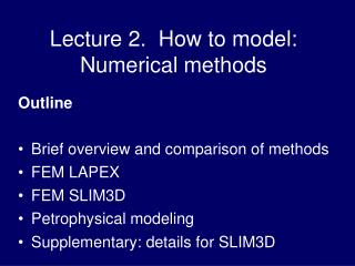
Lecture 2. How to model: Numerical methods. Outline Brief overview and comparison of methods FEM LAPEX FEM SLIM3D Petrophysical modeling Supplementary: details for SLIM3D. Full set of equations. mass. momentum. energy. Final effective viscosity. if. if. Numerical methods.

E N D
Lecture 2. How to model: Numerical methods Outline • Brief overview and comparison of methods • FEM LAPEX • FEM SLIM3D • Petrophysical modeling • Supplementary: details for SLIM3D
Full set of equations mass momentum energy
According to the type of parameterization in time: Explicit, Implicit According to the type of parameterization in space: FDM, FEM, FVM, SM, BEM etc. According to how mesh changes (if) within a deforming body: Lagrangian, Eulerian, Arbitrary Lagrangian Eulerian (ALE)
Brief Comparison of Methods Finite Difference Method (FDM) : FDM approximates an operator (e.g., the derivative) Finite Element Method (FEM) : FEM uses exact operators but approximates the solution basis functions.
Brief Comparison of Methods Spectral Methods (SM): Spectral methods use global basis functions to approximate a solution across the entire domain. Finite Element Methods (FEM): FEM use compact basis functions to approximate a solution on individual elements.
Explicit vrs. Implicit Should be:
Explicit vrs. Implicit Explicit approximation:
Explicit vrs. Implicit Explicit approximation:
Modified FLAC = LAPEX (Babeyko et al, 2002) Dynamic relaxation:
Markers track material and history properties Upper crust Lower crust Mantle
Benchmark: Rayleigh-Taylor instabilityvan Keken et al. (1997)
Friction angle 19° Sand-box benchmark movie Weaker layer
Explicit method vs. implicit • Advantages • Easy to implement, small computational efforts per time step. • No global matrices. Low memory requirements. • Even highly nonlinear constitutive laws are always followed in a valid physical way and without additional iterations. • Strightforward way to add new effects (melting, shear heating, . . . . ) • Easy to parallelize. • Disadvantages • Small technical time-step (order of a year)
Physical background Balance equations Deformation mechanisms Mohr-Coulomb Popov and Sobolev (2008)
Numerical background Discretization by Finite Element Method Arbitrary Lagrangian-Eulerian kinematical formulation Fast implicit time stepping + Newton-Raphson solver Remapping of entire fields by Particle-In-Cell technique Popov and Sobolev (2008)
Solving Stokes equations with code Rhea (adaptive mesh refinement) Burstedde et al.,2008-2010
Solving Stokes equations with code Rhea Stadler et al., 2010
Available from CIG (http://www.geodynamics.org CitComCU. A finite element E parallel code capable of modelling thermo-chemical convection in a 3-D domain appropriate for convection within the Earth’s mantle. Developed from CitCom (Moresi and Solomatov, 1995; Moresi et al., 1996). CitComS.A finite element E code designed to solve thermal convection problems relevant to Earth’s mantle in 3-D spherical geometry, developed from CitCom by Zhong et al.(2000). Ellipsis3D. A 3-D particle-in-cell E finite element solid modelling code for viscoelastoplastic materials, as described in O’Neill et al. (2006). Gale. An Arbitrary Lagrangian Eulerian (ALE) code that solves problems related to orogenesis, rifting, and subduction with coupling to surface erosion models. This is an application of the Underworld platform listed below. PyLith . A finite element code for the solution of viscoelastic/ plastic deformation that was designed for lithospheric modeling problems. SNAC is a L explicit finite difference code for modelling a finitely deforming elasto-visco-plastic solid in 3D. Available from http://milamin.org/. MILAMIN. A finite element method implementation in MATLAB that is capable of modelling viscous flow with large number of degrees of freedom on a normal computer Dabrowski et al. (2008).
Full set of equations mass momentum energy
Full set of equations mass momentum energy
To establish link between rock composition and its physical properties. Direct problems: prediction of the density and seismic structure (also anisotropic) incorporation in the thermomechanical modeling Inverse problem: interpretation of seismic velocities in terms of composition Goals of the petrophysical modeling
Petrophysical modeling Internally-consistent dataset of thermodynamic properties of minerals and solid solutions (Holland and Powell ‘90, Sobolev and Babeyko ’94) Gibbs free energy minimization algorithm After de Capitani and Brown ‘88 SiO2 Al2O3 Fe2O3 MgO + (P,T) CaO FeO Na2O K2O Equilibrium mineralogical composition of a rock given chemical composition and PT-conditions Density and elastic properties optionally with cracks and anisotropy
Vp- density diagram Sobolev and Babeyko, 1994 1- granite, 2- granodiorite, 3- diorite, 4- gabbro, 5- olivine gabbro, 6- pyroxenite, 7,8,9- peridotites
CA arc CA back-arc Vp - Vp/Vs diagram Sobolev and Babeyko, 1994 1- granite, 2- granodiorite, 3- diorite, 4- gabbro, 5- olivine gabbro, 6- pyroxenite, 7,8,9- peridotites
The effect of anelasticity on seismic velocities (Sobolev et al., 1997) Basic relationships which link P and S seismic velocities, temperature, A-parameter, attenuation etc They were obtained from a generalization of different sorts of data: global seismic data, laboratory experiments, and numerical modeling. where: P is pressure, T is the absolute temperature, ω is frequency, Tmelt is melting temperature, Qs and Qp are the S and P- waves quality factors. Values of parameters estimated from laboratory studies and global seismological researches: g=43.8, A=0.0034, α=0.20, Qk=479 (Sobolev et al. 1996)
Supplement: details for FEM SLIM3D (Popov and Sobolev, PEPI, 2008)