Download
1 / 13
130 likes | 202 Views
Detecting Dark Clouds in the Galactic Plane with 2MASS data By : Luis Mercado. In collaboration with the part of GLIMPSE team (Christer Watson, Ed Churchwell and Bob Benjamin). Introduction / Background. What are Dark Clouds and why study them? Optically thick at visual and IR wavelengths

E N D
Detecting Dark Clouds in the Galactic Plane with 2MASS data By : Luis Mercado In collaboration with the part of GLIMPSE team (Christer Watson, Ed Churchwell and Bob Benjamin)
Introduction / Background • What are Dark Clouds and why study them? • Optically thick at visual and IR wavelengths • Star Formation Regions • GLIMPSE & SIRTF • Infrared Surveys • MSX (8 micron) – Showed dark clouds to be thicker than previously believed • 2MASS – 2 Micron All-Sky Survey
2MASS Database • Imaged entire sky in near infrared with J, H & K filters • Used data to produce point source catalog with over 300 million sources • Our selection criteria: • Artifact flags • Magnitude errors < 0.15 mags • Mag limits: • 14.3 for H, 13.5 for K
Our Technique • H-K grid – pixels represent average color excess over a radius of 1.2’ • Stellar density grid – pixels represent number of stars over radius of 1.2’ • Unsharp Masking – used Gaussian to smooth image and create contrast image
Smoothing Process Image - Background _____________________ Contrast = Background 1.2’ radius for image 2.0’ radius for smoothing
Our Technique • H-K grid – pixels represent average color excess over a radius of 1.2’ • Stellar density grid – pixels represent number of stars over radius of 1.2’ • Unsharp Masking – used Gaussian to smooth image and create contrast image • Best technique: product of color and density contrasts
H-Kave from l = 10°-15° H-Kave contrast K stellar density K-density contrast What it all looks like…
Above: Product of density and color contrast. Below: MSX image of same field (l = 10°15°). Notice the correlation between the dark blue objects on the contrast plot and high absorption areas (dark clouds) in the MSX image.
2MASS three color image of test field. Also plotted are contours obtained from our selection method for the corresponding area.
Results / Conclusions • Dark Clouds are identifiable with 2MASS data • Found technique that proves this • Color excess and stellar density are both used as indicators • 380 dark clouds were detected in l = 10°- 40° range with our technique • Since we only see foreground stars, information about the clouds is limited
What Now? • Develop catalogue of Dark Clouds for publishing • Present work at AAS meeting • Use data on future research missions such as SIRTF
Problems Left: Histogram of # of dark clouds detected vs. galactic longitude. Notice a rise in detections at high longitudes, opposite to what would be expected Right: Plot of noise and density versus longitude. Notice the similar behavior. It turns out noise seems to be proportional to the density, but in an unexpected way.