Download
1 / 1
10 likes | 142 Views
Local Hot Bubble (LHB). Loop1 Superbubble. Cosmic Background. Cool Halo. Galactic Bulge. nH (galactic plane). nH (cold column). nH (galactic column). nH (the Wall). Earth. Wabs x Brem (4.0keV). Wabs x Bknpower. Wabs x Apec (0.1keV). Wabs x Vapec (0.3keV). Apec (0.1keV).

E N D
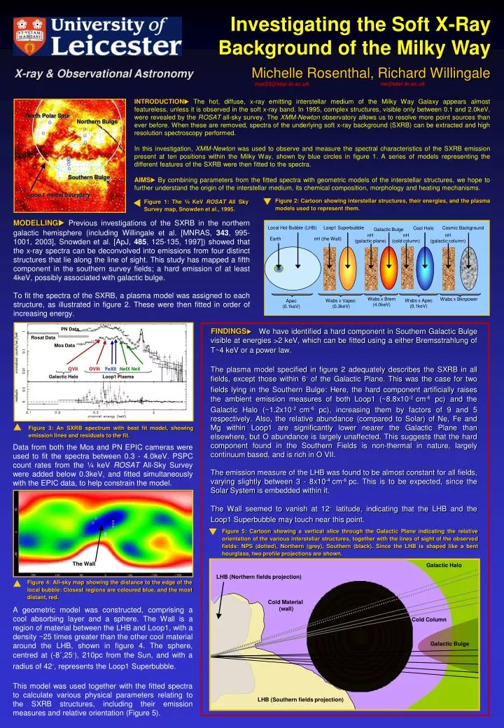
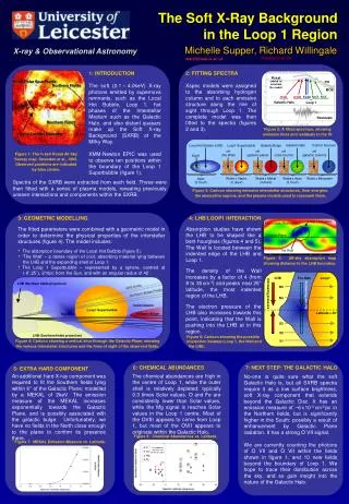
Local Hot Bubble (LHB) Loop1 Superbubble Cosmic Background Cool Halo Galactic Bulge nH (galactic plane) nH (cold column) nH (galactic column) nH (the Wall) Earth Wabs x Brem (4.0keV) Wabs x Bknpower Wabs x Apec (0.1keV) Wabs x Vapec (0.3keV) Apec (0.1keV) PN Data Rosat Data Mos Data OVII OVIIIFeXIINeIX NeX Galactic Halo Loop1 Plasma Galactic Halo LHB (Northern fields projection) The Wall Cold Material (wall) Cold Column Loop1 Superbubble Galactic Bulge LHB (Southern fields projection) Investigating the Soft X-Ray Background of the Milky Way Michelle Rosenthal, Richard Willingale X-ray & Observational Astronomy rw@star.le.ac.uk mar23@star.le.ac.uk INTRODUCTIONu The hot, diffuse, x-ray emitting interstellar medium of the Milky Way Galaxy appears almost featureless, unless it is observed in the soft x-ray band. In 1995, complex structures, visible only between 0.1 and 2.0keV, were revealed by the ROSAT all-sky survey. The XMM-Newton observatory allows us to resolve more point sources than ever before. When these are removed, spectra of the underlying soft x-ray background (SXRB) can be extracted and high resolution spectroscopy performed. In this investigation, XMM-Newton was used to observe and measure the spectral characteristics of the SXRB emission present at ten positions within the Milky Way, shown by blue circles in figure 1. A series of models representing the different features of the SXRB were then fitted to the spectra. AIMSu By combining parameters from the fitted spectra with geometric models of the interstellar structures, we hope to further understand the origin of the interstellar medium, its chemical composition, morphology and heating mechanisms. North Polar Spur Northern Bulge Southern Bulge Loop 1 model boundary q Figure 2: Cartoon showing interstellar structures, their energies, and the plasma models used to represent them. t Figure 1: The ¾ KeV ROSAT All Sky Survey map, Snowden et al., 1995. MODELLINGuPrevious investigations of the SXRB in the northern galactic hemisphere (including Willingale et al. [MNRAS, 343, 995-1001, 2003], Snowden et al. [ApJ, 485, 125-135, 1997]) showed that the x-ray spectra can be deconvolved into emissions from four distinct structures that lie along the line of sight. This study has mapped a fifth component in the southern survey fields; a hard emission of at least 4keV, possibly associated with galactic bulge. To fit the spectra of the SXRB, a plasma model was assigned to each structure, as illustrated in figure 2. These were then fitted in order of increasing energy. FINDINGSu We have identified a hard component in Southern Galactic Bulge visible at energies >2 keV, which can be fitted using a either Bremsstrahlung of T~4 keV or a power law. The plasma model specified in figure 2 adequately describes the SXRB in all fields, except those within 6˚ of the Galactic Plane. This was the case for two fields lying in the Southern Bulge: Here, the hard component artificially raises the ambient emission measures of both Loop1 (~8.8x10⁻² cm-6pc)and the Galactic Halo (~1.2x10⁻² cm-6 pc), increasing them by factors of 9 and 5 respectively. Also, the relative abundance (compared to Solar) of Ne, Fe and Mg within Loop1 are significantly lower nearer the Galactic Plane than elsewhere, but O abundance is largely unaffected. This suggests that the hard component found in the Southern Fields is non-thermal in nature, largely continuum based, and is rich in O VII. The emission measure of the LHB was found to be almost constant for all fields, varying slightly between 3 - 8x10⁻⁴ cm-6 pc. This is to be expected, since the Solar System is embedded within it. The Wall seemed to vanish at 12˚ latitude, indicating that the LHB and the Loop1 Superbubble may touch near this point. p Figure 3: An SXRB spectrum with best fit model, showing emission lines and residuals to the fit. Data from both the Mos and PN EPIC cameras were used to fit the spectra between 0.3 - 4.0keV. PSPC count rates from the ¼ keV ROSAT All-Sky Survey were added below 0.3keV, and fitted simultaneously with the EPIC data, to help constrain the model. q Figure 5: Cartoon showing a vertical slice through the Galactic Plane indicating the relative orientation of the various interstellar structures, together with the lines of sight of the observed fields: NPS (dotted), Northern (grey), Southern (black). Since the LHB is shaped like a bent hourglass, two profile projections are shown. p Figure 4: All-sky map showing the distance to the edge of the local bubble: Closest regions are coloured blue, and the most distant, red. A geometric model was constructed, comprising a cool absorbing layer and a sphere. The Wall is a region of material between the LHB and Loop1, with a density ~25 times greater than the other cool material around the LHB, shown in figure 4. The sphere, centred at (-8˚,25˚), 210pc from the Sun, and with a radius of 42˚, represents the Loop1 Superbubble. This model was used together with the fitted spectra to calculate various physical parameters relating to the SXRB structures, including their emission measures and relative orientation (Figure 5).


![[ Michelle Kolbe]](https://cdn3.slideserve.com/6861681/slide1-dt.jpg)