Download
1 / 7
70 likes | 169 Views
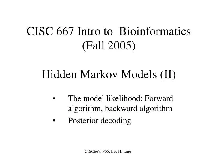
CISC 667 Intro to Bioinformatics (Fall 2005) Hidden Markov Models (II). The model likelihood: Forward algorithm, backward algorithm Posterior decoding. 0.70. 0.65. A: .170 C: .368 G: .274 T: .188. A: .372 C: .198 G: .112 T: .338. 0.35. 0.30. +. −.

E N D
CISC 667 Intro to Bioinformatics(Fall 2005)Hidden Markov Models (II) The model likelihood: Forward algorithm, backward algorithm Posterior decoding CISC667, F05, Lec11, Liao
0.70 0.65 A: .170 C: .368 G: .274 T: .188 A: .372 C: .198 G: .112 T: .338 0.35 0.30 + − The probability that sequence x is emitted by a state path π is: P(x, π) = ∏i=1 to Leπi (xi) a πi πi+1 i:123456789 x:TGCGCGTAC π :--++++--- P(x, π) = 0.338 ×0.70 × 0.112 × 0.30 × 0.368 × 0.65 × 0.274 × 0.65 × 0.368 × 0.65 × 0.274 × 0.35 × 0.338 × 0.70 × 0.372 × 0.70 × 0.198. Then, the probability to observe sequence x in the model is P(x) = π P(x, π), which is also called the likelihood of the model. CISC667, F05, Lec11, Liao
x1 x2 x3 xL 1 1 1 1 0 0 N N N N How to calculate the probability to observe sequence x in the model? P(x) = π P(x, π) Let fk(i) be the probability contributed by all paths from the beginning up to (and include) position i with the state at position i being k. The the following recurrence is true: f k(i) = [ j f j(i-1) ajk ] ek(xi) Graphically, Again, a silent state 0 is introduced for better presentation CISC667, F05, Lec11, Liao
Forward algorithm • Initialization: f0(0) =1, fk(0) = 0 for k > 0. • Recursion: fk(i) = ek(xi) jfj(i-1) ajk. • Termination: P(x) = kfk(L) ak0. • Time complexity: O(N2L), where N is the number of states and L is the sequence length. CISC667, F05, Lec11, Liao
Let bk(i) be the probability contributed by all paths that pass state k at position i. • bk(i) = P(xi+1, …, xL | (i) = k) • Backward algorithm • Initialization: bk(L) = ak0 for all k. • Recursion (i = L-1, …, 1): bk(i) = j akjek(xi+1) fj(i+1). • Termination: P(x) = k a0k ek(x1)bk(1). • Time complexity: O(N2L), where N is the number of states and L is the sequence length. CISC667, F05, Lec11, Liao
Posterior decoding P(πi = k |x) = P(x, πi = k) /P(x) = fk(i)bk(i) / P(x) Algorithm: for i = 1 to L do argmax k P(πi = k |x) Notes: 1. Posterior decoding may be useful when there are multiple almost most probable paths, or when a function is defined on the states. 2. The state path identified by posterior decoding may not be most probable overall, or may not even be a viable path. CISC667, F05, Lec11, Liao
The log transformation for Viterbi algorithm vk(i) = ek(xi) maxj(vj(i-1) ajk); ajk = log ajk; ek(xi) = log ek(xi); vk(i) = log vk(i); vk(i) = ek(xi) + maxj(vj(i-1) + ajk); CISC667, F05, Lec11, Liao