Download

1 / 13
130 likes | 245 Views
CISC 667 Intro to Bioinformatics (Spring 2007) Phylogenetic Trees (III). Probabilistic methods. x 5. t 4. t 3. 2. x 4. t 2. t 1. x 2. x 1. x 3. Bayes rule revisited. P(model|data) = P(data|model) P(model)/P(data) model includes our evolution theory,

E N D
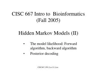
CISC 667 Intro to Bioinformatics(Spring 2007)Phylogenetic Trees (III) Probabilistic methods CISC667, S07, Lec18, Liao
x5 t4 t3 2 x4 t2 t1 x2 x1 x3 Bayes rule revisited. P(model|data) = P(data|model) P(model)/P(data) • model includes • our evolution theory, • a specific phylogenetic tree (topology and edge lengths), and • assignment of sequences to the tree leaves. • Data: a set of sequences that are used to infer phylogeny. Let P(x|y, t) be the probability in that sequence x is evolved from an ancestral sequence y over an edge of length t. P( x1, x2, x3, x4, x5|T, t.) = P( x1| x4, t1) P( x2| x4, t2) P( x3| x5, t3) P( x4| x5, t4) P( x5) A shorthand notation P( x·|T, t.) is used where x· stands for a set of sequences, and t. for edge lengths of the tree T. CISC667, S07, Lec18, Liao
In general, if we know • P(x|y, t) for any x, y, and t • A tree T, and assignment of sequences to tree nodes, Then we can compute the likelihood for observing the sequences as they are assigned onto the tree leaves. Q: Given n, the number of leaves, there are (2n-3)!! different trees (plus many different ways to assign length to tree edges), which tree can best interpret the data? A: The tree that gives the maximum likelihood (ML). In practice, to implement the ML method, two issues we need to address • A model of evolution, which gives the conditional probabilities P(x|y, t) • Method to find the maximum likelihood. For this, any optimization method may be utilized, such as • Descent gradient • Simulated annealing • Genetic algorithm CISC667, S07, Lec18, Liao
P(A|A, t) P(A|C, t) P(A|G, t) P(A|T, t) P(C|A, t) P(C|C, t) P(C|G, t) P(C|T, t) S(t) = P(G|A, t) P(G|C, t) P(G|G, t) P(G|T, t) P(T|A, t) P(T|C, t) P(T|G, t) P(T|T, t) Models of evolution Independence assumption: mutations occur independently at different positions. Therefore, P(x|y, t) = u P(xu|yu, t), where P(xu|yu, t) is the probability that residue xu in sequence x mutates to residue yu in sequence y over time t. multiplicative assumption: P(b|a, t + t) = c P(c|a, t)·P(b|c, t). For DNA sequences, probabilities for all possible mutations among four nucleotides during a given time period t form a 4 by 4 matrix And, we have multiplicative property for these matrices S(t) ·S(t) = S(t + t). CISC667, S07, Lec18, Liao
1-3r r r r r 1-3r r r S(t)= r r 1-3r r t I + R t r r r 1-3r 1 0 0 0 For each P(b|a, t) in the substitution matrix S(t), it is reasonable to assume that no mutation can occur at zero time interval: • P(a|a, 0) = 1 • P(b|a, 0) = 0. That is, Further, let’s assume that P(b|a, t) over a infinitesimal interval t is proportional to t by a constant r, called mutation rate: P(b|a, t) = r t. Jukes-Cantor model for DNA sequences assumes that all nucleotide mutations have the same rate. That is, 0 1 0 0 S(0) = 0 0 1 0 0 0 0 1 CISC667, S07, Lec18, Liao
Therefore, S(t + t) = S(t) ·S(t) = S(t) ·[I + Rt] [S(t + t) - S(t)] /t = S(t)·R S’(t) = S(t)·R when t 0. Solving the differential equations, we have • P(a|a, t) = ¼ (1+ 3e -4rt) for a {A,C, G, T} • P(b|a, t) = ¼ (1- e -4rt) for ab, a and b {A,C, G, T} In this model, when t = , P(b|a, ) = ¼. That is, the nucleotide equilibrium frequencies are all equal. CISC667, S07, Lec18, Liao
1-2r-s r s r r 1-2r-s r s S(t)= s r 1-2r -s r r s r 1-2r-s A C G T Kimura model for DNA sequences assumes different rates for transitions (AG and C T) and transversions (A T, G T, A C, and C G). That is, Similar models are proposed for mutations among amino acids. If we were able to quantify the “time” as how many number mutations have occurred, the substitute matrices in those models would correspond to PAM matrices at respective times. A C G T t I+R t CISC667, S07, Lec18, Liao
Maximum Likelihood t2 t1 • The case of two sequences aligned with no gaps P( x1, x2|T, t1, t2) = u=1 to NP( x1u, x2u|T, t1, t2) • Let x1 = CCGGCCGCGCG x2 = CGGGCCGCCCG P(C,C| T, t1, t2) = P(C|A, t2) P(C|A, t1) P(A) + P(C|C, t2) P(C|C, t1) P(C) + P(C|G, t2) P(C|G, t1) P(G) + P(C|T, t2) P(C|T, t1) P(T) = ¼ [3 ¼ (1- e -4rt1) ¼ (1- e -4rt2) + ¼ (1+3 e -4rt1) ¼ (1+3 e -4rt2) ] = 1/16 (1+3 e -4r(t1 +t2)). P(C,G| T, t1, t2) = 1/16 (1- e -4r(t1 +t2)). Therefore, for an alignment that has n1 identical sites and n2 mutational sites, we have P( x1, x2|T, t1, t2) = 1/ 16n1+n2(1+3 e -4r(t1 +t2))n1 (1- e -4r(t1 +t2))n2, which is a function of edge lengths in tree T. x2 x1 CISC667, S07, Lec18, Liao
P = 0 t tm In general, the probability can be computed by working up the tree from the leaves using post-order traversal. This is done by Felsenstein’s algorithm (1981). Once the probability is available, optimizing the assignments of edge lengths t in the tree amounts to Where tm is the tree length assignment that maximize the likelihood. CISC667, S07, Lec18, Liao
How to optimize tree topology? • Discrete structure, therefore cannot take derivatives. Basic strategy for searching the tree space • A tree generation algorithm that can generate trees • Assess the likelihood • Accept • Reject A genetic algorithm implementation [Matsuda 1998] CISC667, S07, Lec18, Liao
Genetic algorithm Input • P, the population, • r: the fraction of population to be replaced, • f, a fitness, • ft, the fitness_threshold, • m: the rate for mutation. Initialize population (randomly) Evaluate: for each h in P, compute Fitness(h) While [Maxh f(h)] < ft do • Select • Crossover • Mutate • Update P with the new generation Ps • Evaluate: f(h) for all h P Return the h in P that has the best fitness CISC667, S07, Lec18, Liao
Key components for implementing genetic algorithms • Representing hypotheses (which are the trees here) • New Hampshire format (A,(F,(C,(B,D)))) • Genetic operators • Crossover: • Single • Two point • uniform • Mutation: point • Fitness function: we use the likelihood computed for each tree using F C B D A CISC667, S07, Lec18, Liao
More advanced topics in phylogenetic analysis • Different heuristics for sampling the tree space • Monte Carlo • … • More realistic evolutionary models • With gaps • Non-uniform: different rates at different sites • … • Using different data sets and reconciliation • Sequences • Gene positions [Nadeau & Taylor 1984, PNAS 81:814-818, Pavzner, Sankoff, …] • … CISC667, S07, Lec18, Liao