Download
1 / 58
580 likes | 717 Views
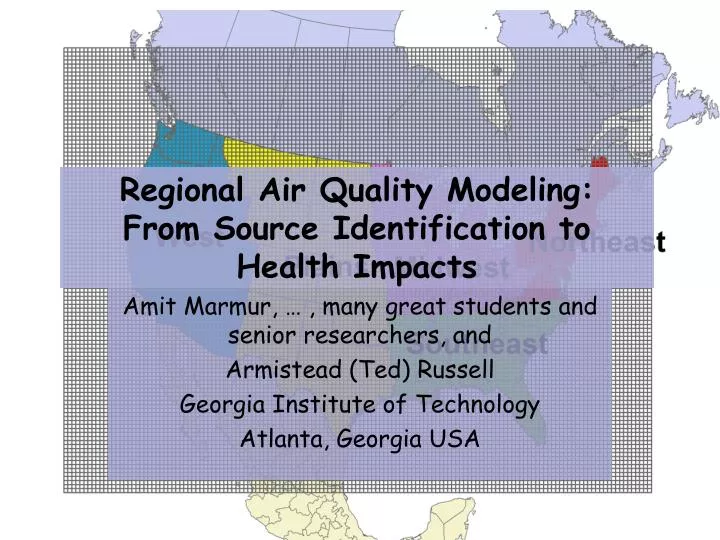
Regional Air Quality Modeling: From Source Identification to Health Impacts. Amit Marmur, … , many great students and senior researchers, and Armistead (Ted) Russell Georgia Institute of Technology Atlanta, Georgia USA. With Special Thanks to:. Paige Tolbert and the Emory crew

E N D
Regional Air Quality Modeling:From Source Identification to Health Impacts Amit Marmur, … , many great students and senior researchers, and Armistead (Ted) Russell Georgia Institute of Technology Atlanta, Georgia USA
With Special Thanks to: • Paige Tolbert and the Emory crew • As part of ARIES, SOPHIA, and follow on studies • NIEHS, US EPA, FHWA, Southern Company, SAMI • Financial assistance • JGSEE of Thailand • And more…
Issues • Approximately 799,000 excess deaths per year occur per year due to air pollution • 487,000 in Asia (S, SE and W. Pacific) • Variety of health impacts in Thailand tied to air pollutants • Primarily due to: • PM2.5: small particles, Range of health impacts, visibility impairment, … • Ozone • PAPA Studies show strong associations with PM and ozone in Asia • Most of PM2.5 burden comes from combustion to transform energy • Primary and secondary emissions • Need reliable approaches to identify how energy sources impact air quality: Source Apportionment • Air quality management • Health impact assessment
Ozone Formation h (sunlight) Ozone Isopleth ENOx NOx oxides of nitrogen (NO + NO2) High O3 O3 Low O3 EVOC VOCs Volatile organic compounds
PM Formation h (sunlight) SO2 Sulfur dioxide PM NOx VOCs, OC & EC
Particulate Matter • Complex mixture of solid and liquid particles suspended in the ambient air • Size classifications • “super-coarse” > 10μm • “coarse” (PM10) < 10μm • “fine” (PM2.5) < 2.5μm • “ultrafine” < 0.1μm • Many sources • Many chemical species:
Fine Particles: Why should we care ? RESPIRATORY EFFECTS CARDIOVASCULAR EFFECTS Effects on Lung Function Effects on Cardiovascular Function Airway Inflammation Vascular Inflammation Image courtesy of the U.S. EPA
Outline • Atmospheric modeling • Types • Basics • Approaches • Advanced approaches • Applications • Source impacts • health impact assessment
Emissions- Based Hybrid Receptor CMB FA Lag. Eulerian (grid) PMF Molec. Mark. Norm. Source Specific* “Mixed PM” UNMIX PM (Source Apportionment) Models(those capable of providing some type of information as to how specific sources impact air quality) PM Models Statistical First-principle
Role of Atmospheric Modeling In Air Quality Assessment Air Quality Goals Air Quality/Health Impacts Controls Pollutant Distributions Air Quality Model or Emissions
Receptor Models Obsserved Air Quality Ci(t) Source Impacts Sj(t) Ci - ambient concentration of specie i (g/m3) fi,j - fraction of specie i in emissions from source j Sj - contribution (source-strength) of source j (g/m3)
Receptor Models • Strengths • Results tied to observed air quality • Less resource intensive (provided data is available) • Weaknesses • Data dependent (accuracy, availability, quantity, etc.) • Monitor • Source characteristics • Not apparent how to calculate uncertainties • Do not add “coverage” directly
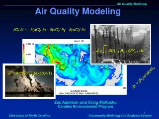
Chemistry Emissions-based Air Quality Model • Representation of physical and chemical processes • Numerical integration routines • Scientifically most sound method to link future emissions changes to air quality Computational Planes 5-20 50-100 50-200 Air Quality Model Atmospheric Diffusion Equation Numerics C=AxB+E Discretize Emissions Meteorology Operator splitting 200 species x 10000 hor. grids x 20 layers= 40 million coupled, stiff non-linear differential equations
Heterogeneous Processes Homogeneous Processes Chemistry and Aerosol Dynamics Photochemical Reactions Aerosol Dynamics Thermochemical Reactions Chemical Processes (R) Surface Deposition Sink Processes Sources Emissions 1. Anthropogenic 2. Geogenic 3. Biogenic Air Quality Numerical Solution Techniques Computed Concentrations Sources (E,S, BCs) Transported Pollutants Meteorology Transport (U, K, Vd) Radiation Temperature Topography & Land use Turbulence Geographical Features Cloud Cover Wind Air Quality Model
Chemical Mechanism Specification Air Quality Model Chemical Mechanism Historical: Specified Evolving: Compiler Model Evaluation Emissions Inputs Historical: NO, NO2, HONO Lumped VOCs CO, SO2 Evolving: PM, NH3, Detailed VOCs, Adv. Biogenics Numerical Routines Historical: Advection Chem. Kinet. Evolving Sens. Anal. Proc. Integ. Unc. Anal. Pollutant Distributions Evolving: Sensitivities Uncertainties Model Parameter Calculation Emissions Model Inputs: Emissions Inventory Population Roads Land Use Industry Meteorology Meteorological Inputs Historical 2- or 3-D winds; Ground level T, RH; Mixing height, Land use Evolving: 3-D Winds, Diffusivities, Temp., RH, D, Solar Insolation (UV & total solar)... Temperature, Solar Insolation Emissions Inventory Development Air Quality Data Analysis and Processing Meteorological Model (Diagnostic or Prognostic) Topographical Data Meteorological Observations Emissions, Industry and Human Activity Data Air Quality Observations Foundation Atmospheric Modeling Process
Grids Adaptive (Odman et al.) Nested About 15 vertical Layers up to 15 km (many in first 1 km) Multiscale (Odman et al.)
How well do they work?* *Performance relies on quality of inputs. US has spent decades on emissions inventory development. Meteorological modeling also contributes significantly to errors
Source-based Models • Strengths • Direct link between sources and air quality • Provides spatial, temporal and chemical coverage • Weaknesses • Result accuracy limited by input data accuracy (meteorology, emissions…) • Resource intensive
Hybrid: Inverse Model Approach* INPUTS Emissions (Eij(x,t)) Ci(x,t), Fij(x,t), & Sj(x,t) Air Quality Model + DDM-3D Other Inputs Receptor Model New emissions: Eij(x,t) Observations taken from routine measurement networks or special field studies Main assumption in the formulation: A major source for the discrepancy between predictions and observations are the emission estimates
What’s next? • Emissions-based air quality models work pretty well, how might we use them: • Identify, quantitatively, how specific sources impact air quality. • Develop and test control strategies • Decoupled direct method (implemented in CIT, URM, MAQSIP, CMAQ, CAMX) • Dunker: initial applications • Yang et al.: large scale application, comp. efficient (CIT, URM) • Hakami et al. ,Cohan et al: Higher order, with applications (MAQSIP, CMAQ) • Napelenok eet al., : PM • Control strategy assessment • Least cost approach to attainment for Macon, GA (Cohan et al.) • Assessing impacts of individual sources • Area of Influence analysis (AOI) (similar information as developing the adjoint) • Or AOPI (potential influence) • Application to health assessment
Example Results : Impact of Planned Controls: 2000 vs. 2007 Emissions reductions lead to about a 12 ppb ozone reduction: Atlanta and Macon do not attain ozone standard (Macon by 6ppb)
Model Parameters (P) State Variables: Sensitivity Parameters: Inputs (P) Model Sensitivity analysis • Given a system, find how the state (concentrations) responds to incremental changes in the input and model parameters: If Pj are emissions, Sij are the sensitivities/responses to emission changes, e.g.., the sensitivity of ozone to Atlanta NOx emissions
Advection Diffusion Chemistry Emissions Sensitivity Analysis with Decoupled Direct Method (DDM): The Power of the Derivative • Define first order sensitivities as • Take derivatives of • Solve sensitivity equations simultaneously
DDM-3D NOo NO2o VOCio ... T K u, v, w Ei ki BCi ... 3-D Air Quality Model O3(t,x,y,z) NO(t,x,y,z) NO2(t,x,y,z) VOCi(t,x,y,z) ... decoupled DDM-3D Sensitivity Analysis J
CA CB EB EA DDM compared to Brute Force Sulfate Emissions of SO2
Consistency of first-order sensitivities Brute Force (20% change) DDM-3D R2 > 0.99 Low bias & error
Advantages of DDM-3D • Computes sensitivities of all modeled species to many different parameters in one simulation • Can “tell” model to give sensitivities to 10s of parameters in the same run • Captures small perturbations in input parameters • Strangely wonderful • Avoids numerical errors sometimes present in sensitivities calculated with Brute Force • Lowers the requirement for computational resources
Evidence of Numerical Errors in BF NH4 sensitivity to domain-wide SO2 reductions NOx reductions at a point
Control Strategy Development • Macon out of attainment by 6 ppb in 2007 • Want to identify least cost control strategy • Process: • Identify possible controls and costs ($/ton of VOC or NOx) • Simulate response to controls (D[O3]/ton VOC or NOx) • Calculate control effectiveness(D[O3]/$) • Choose most effective controls until get 6 ppb • Test strategy
Macon Scherer Sources of Macon’s ozone A B S M Atlanta Branch 8-hr ozone, Aug. 17, 2000 (2007 emissions)
2007 Emissions and Sensitivities NOx emission rates (tpd) Macon ozone sensitivity (ppt/tpd)
Marginal Abatement Costs by Region Cost Cost-optimization Choose options with least marginal $/impact until: (1) attain a.q. goal, or (2) reach budget constraint Impact Source-Receptor Response
Strategies for Macon attainment (need 6.5 ppb) • Key Measures • Zero-cost options (PRB coal, burning ban, ...): 1.72 ppb, $0 • Bibb industrial NOx: 0.82 ppb, $2.6 million • Locomotive controls: 0.77 ppb, $7.3 million • SCRs at Scherer: 1.63 ppb, $20.9 million • Vehicle I&M in Bibb: • 0.25 ppb, $4.9 million
Single-Source Impact Analysis (Bergin et al.) Provide a technique to evaluate the impacts from a single large emissions source on regional air quality, incorporating non-linear processes and multi-day effects in estimating pollutant responses to relatively small emissions perturbations.
Motivation and Application • The ability to evaluate regional secondary pollution impacts from large single sources would provide a valuable tool for more effective air quality management practices, such as refining programs (e.g. emissions trading, regional planning), and supporting more effective compliance enforcement. • Typical modeling approach (removing the emissions from a single source) has numerical errors. • Court case led to need to assess impact of a single power plant (Sammis) in Ohio on downwind areas (a distance of up to about 1000 km)
Average Day Elevated NOx Emissions 2500 2000 1500 NOx Emissions (avg tons/day) 1000 excess 500 allowable 0 Ohio Elevated EGU Jul-95 Model Inventory May-95 Jul-95 Aug-00 W. H. Sammis Power Plant(court estimated emissions) Court Estimated from W.H. Sammis Plant
CMAQ, 36x36 kmAug. 12-20, 20002-ord. DDM URM, multiscale from 24x24 km2July 11-19 and May 24-29, 1995 DDM Approach Two air quality models and grids, three ozone episodes, and three sensitivity techniques (brute-force, DDM, higher order DDM)
Maximum increase in 1-hr avg O3 Comparison of the maximum increase in hourly-averaged ozone concentrations due to excess NOx emissions from the Sammis plant. CMAQ with 2nd order DDM URM with DDM • July 11-19, 1995 (b) May 24-29, 1995 (c) August 12-20, 2000
maximum = 2.2 maximum = 2.2 minimum = -1.2 minimum = -3.6 1-hr O3 cell responses to excess emissions All hours When O3 > 0.060 ppm Max. increases Max.decreases CMAQ, 2nd ord DDM, August
Conclusions • Single-source simulation results agree with past field experiments, indicating that appropriate modeling techniques are available for quantifying single-source regional air quality impacts.
Air Quality Models and Health Impact Assessment • (How) Can we use “air quality models” to help identify associations between ozone PM sources and health impacts? • Species vs. sources • Very different than for traditional air quality management
Epidemiology • Identify associations between air quality metrics and health endpoints: Health endpoints Statistical Analysis Sulfate Association
Exposure: daily PM2.5 (mg/m3); lag 0, 1, 2 Outcome: daily ED visit counts for CVD 70 35 0 140 70 0 1998 2001 2004 1998 2001 2004 Epidemiologic Analysis log{E(CVD)} = a + b [PM2.5] + covariate terms Covariates: time trend (mo. knots), day-of-week, holidays, hospital entry/exit, temperature, dew point
Association between CVD Visits and Air Quality (Tolbert et al., 2004)
Issues • May not be measuring the species primarily impacting health • Observations limited to subset of compounds present • Many species are correlated • Inhibits correctly isolating impacts of a species/primary actors • Inhibits identifying the important source(s) • Observations have errors • Traditional: Measurement is not perfect • Representativeness (is this an error? Yes, in an epi-sense) • Observations are sparse • Limited spatially and temporally • Multiple pollutants may combine to impact health • Statistical models can have trouble identifying such phenomena • Ultimately want how a source impacts health • We control sources
Health Endpoints Statistical Analysis Use AQ Models to Address Issues: Link Sources to Impacts Data Air Quality Model Source Impacts S(x,t) Association between Source Impact and Health Endpoints
Source Impacts on Air Quality(Nov 1998 – Aug 2000) CMB Source Impacts