Download
1 / 9

E N D
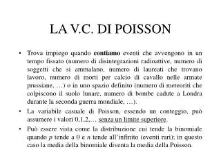
LA V.C. DI POISSON • Trova impiego quando contiamo eventi che avvengono in un tempo fissato (numero di disintegrazioni radioattive, numero di soggetti che si ammalano, numero di laureati che trovano lavoro, numero di morti per calcio di cavallo nelle armate prussiane, …) o in uno spazio definito (numero di meteoriti che colpiscono il suolo lunare, numero di bombe cadute a Londra durante la seconda guerra mondiale, …). • La variabile casuale di Poisson, essendo un conteggio, può assumere i valori 0,1,2,… senza un limite superiore. • Può essere vista come la distribuzione cui tende la binomiale quando p tende a 0 e n tende all’infinito (eventi rari); in questo caso la media della binomiale diventa la media della Poisson.
LA V.C. DI POISSON In un esperimento poissoniano, la distribuzione del numero di eventiX è la distribuzione di Poisson con parametrom: La media di una variabile casuale di Poisson è m. La varianza di una variabile casuale di Poisson è m.
ALCUNI ESEMPI CON R • La funzione che chiamiamo è Poisson (con un parametro); notare la maiuscola iniziale • Vediamo cosa succede al variare di m.
LA V.C. DI POISSON • La distribuzione di Poisson è sempre asimme-trica positiva. • Al crescere della media, pur rimanendo asim-metrica, la distribuzione tende sempre di più a concentrarsi in una zona intorno alla media. • Al crescere della media, la distribuzione di Poisson tende alla normale (con media m e varianza m).
LA V.C. DI POISSON • The classic Poisson example is the data set of von Bortkiewicz (1898), for the chance of a Prussian cavalryman being killed by the kick of a horse. • Ten army corps were observed over 20 years, giving a total of 200 observations of one corps for a one year period. • The period or module of observation is thus one year. • The total deaths from horse kicks were 122, and the average number of deaths per year per corps was thus 122/200 = 0.61. • In any given year, we expect to observe sometimes none, sometimes one, occasionally two, perhaps once in a while three, and (we might intuitively expect) very rarely any more. • Here, then, is the classic Poisson situation: a rare event, whose average rate is small, with observations made over many small intervals of time.
LA V.C. DI POISSON > Poisson(122/200) mu: 0.61 Valore atteso (media) : 0.61 Varianza : 0.61 Somma delle probabilita': 1 x f(x) F(x) [1,] 0 5.433509e-01 0.5433509 [2,] 1 3.314440e-01 0.8747949 [3,] 2 1.010904e-01 0.9758853 [4,] 3 2.055505e-02 0.9964404 [5,] 4 3.134646e-03 0.9995750 [6,] 5 3.824268e-04 0.9999575
LA V.C. DI POISSON > x <- c(0,1,2,3,4) > n <- c(109,65,22,3,1) > (mu <- sum(x*n)/sum(n)) [1] 0.61 > fatt <- dpois(x,mu)*sum(n) > cbind(x,n,round(fatt,1)) x n [1,] 0 109 108.7 [2,] 1 65 66.3 [3,] 2 22 20.2 [4,] 3 3 4.1 [5,] 4 1 0.6 > sum(fatt) [1] 199.915
LA V.C. DI POISSON > foss <- c(n[1:3],n[4]+n[5]) > fatt <- c(fatt[1:3],sum(n)-sum(fatt[1:3])) > cbind(foss,round(fatt,1)) foss [1,] 109 108.7 [2,] 65 66.3 [3,] 22 20.2 [4,] 4 4.8 > sum((foss-fatt)^2/fatt) [1] 0.3235236