Download
1 / 38
380 likes | 386 Views
This chapter discusses the origin of magnetic fields due to moving charges and how to calculate the magnetic field at a point using the Biot-Savart law. It also covers the force between two current-carrying conductors and introduces Ampère's law for highly symmetric configurations.

E N D
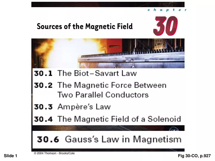
we discussed the magnetic force exerted on a charged particle moving in a magnetic field. • To complete the description of the magnetic interaction, this chapter deals with the origin of the magnetic field—moving charges. We begin by showing how to use the law of Biot and Savart to calculate the magnetic field produced at some point in space by a small current element.
Using this formalism and the principle of superposition, we then calculate the total magnetic field due to various current distributions. • Next, we show how to determine the force between two current-carrying conductors, which leads to the definition of the ampere. • We also introduce Ampère’s law, which is useful in calculating the magnetic field of a highly symmetric configuration carrying a steady current.
Jean-Baptiste Biot (1774–1862) and Félix Savart (1791–1841) performed quantitative experiments on the force exerted by an electric current on a nearby magnet. The magnetic field dB at a point due to the current I through a length element ds is given by the Biot–Savart law. The direction of the field is out of the page at P and into the page at P. Fig 30-1, p.927
• The vector dB is perpendicular both to ds (which points in the direction of the current) and to the unit vector - r directed from ds to P. • The magnitude of dB is inversely proportional to r2, where r is the distance from ds to P. • The magnitude of dB is proportional to the current and to the magnitude ds of the length element ds. • The magnitude of dB is proportional to sinθ, where θ is the angle between the vectors ds and ˆr.
To find the total magnetic field B created at some point by a current of finite size, we must sum up contributions from all current elements Ids that make up the current. That is, we must evaluate B by integrating Equation 30.1
Consider a thin, straight wire carrying a constant current I and placed along the x axis as shown in Figure …. Determine the magnitude and direction of the magnetic field at point P due to this current Fig 30-3, p.929
The right-hand rule The right-hand rule for determining the direction of the magnetic field surrounding a long, straight wire carrying a current. Note that the magnetic field lines form circles around the wire. Fig 30-4, p.930
(a) Magnetic field lines surrounding a current loop. (b) Magnetic field lines surrounding a current loop, displayed with iron filings. (c) Magnetic field lines surrounding a bar magnet. Note the similarity between this line pattern and that of a current loop Fig 30-7, p.931
Consider two long, straight, parallel wires separated by a distance a and carrying currents I1 and I2 in the same direction • We can determine the force exerted on one wire due to the magnetic field set up by the other wire. • parallel conductors carrying currents in the same direction attract each other, and parallel conductors carrying currents in opposite directions repel each other. Fig 30-8, p.932
Because the magnitudes of the forces are the same on both wires, we denote the magnitude of the magnetic force between the wires as simply FB . • We can rewrite this magnitude in terms of the force per unit length Andre-Marie Ampère French Physicist (1775–1836)
Because the compass needles point in the direction of B, we conclude that the lines of B form circles around the wire, • the magnitude of B is the same everywhere on a circular path centered on the wire and lying in a plane perpendicular to the wire. • By varying the current and distance a from the wire, we find that B is proportional to the current and inversely proportional to the distance from the wire, Fig 30-9ab, p.933
Ampère’s law describes the creation of magnetic fields by all continuous current configurations, but at our mathematical level it is useful only for calculating the magnetic field of current configurations having a high degree of symmetry. Its use is similar to that of Gauss’s law in calculating electric fields for highly symmetric charge distributions. Fig 30-9a p.933
Let us choose for our path of integration circle 1 in Figure …From symmetry, B must be constant in magnitude and parallel to ds at every point on this circle. Because the total current passing through the plane of the circle is I0, Ampère’s law gives
Now consider the interior of the wire, where r <R. Here the current I passing through the plane of circle 2 is less than the total current I 0 . Because the current is uniform over the cross-section of the wire, the fraction of the current enclosed by circle 2 must equal the ratio of the area r 2 enclosed by circle 2 to the cross-sectional area R2 of the wire:
A solenoid is a long wire wound in the form of a helix. With this configuration, a reasonably uniform magnetic field can be produced in the space surrounded by the turns of wire—which we shall call the interior of the solenoid—when the solenoid carries a current. • the field lines in the interior are nearly parallel to one another, are uniformly distributed, and are close together, indicating that the field in this space is uniform and strong. * The magnetic field lines for a loosely wound solenoid.
The field lines between current elements on two adjacent turns tend to cancel each other because the field vectors from the two elements are in opposite directions. • The field at exterior points such as P is weak because the field due to current elements on the right-hand portion of a turn tends to cancel the field due to current elements on the left-hand portion.
Magnetic field lines for a tightly wound solenoid of finite length, carrying a steady current • The field at exterior points such as P is weak because the field due to current elements on the right-hand portion of a turn tends to cancel the field due to current elements on the left-hand portion. The magnetic field pattern of a bar magnet, displayed with small iron filings on a sheet of paper. Fig 30-18a, p.938
An ideal solenoid is approached when the turns are closely spaced and the length is much greater than the radius of the turns. In this case, the external field is zero, and the interior field is uniform over a great volume.
Because the solenoid is ideal, B in the interior space is uniform and parallel to the axis, and B in the exterior space is zero. Consider the rectangular path of length and width w shown in Figure…. We can apply Ampère’s law to this path by evaluating the integral of B.ds over each side of the rectangle.
valid only for points near the center (that is, far from the ends) of a very long solenoid. If the radius r of the torus in Figure 30.13 containing N turns is much greater than the toroid’s cross-sectional radius a, a short section of the toroid approximates a solenoid for which
Consider the special case of a plane of area A in a uniform field B that makes an angle θ with dA. The magnetic flux through the plane in this case is
A rectangular loop of width a and length b is located near a long wire carrying a current I (Fig. 30.21). The distance between the wire and the closest side of the loop is c . The wire is parallel to the long side of the loop. Find the total magnetic flux through the loop due to the current in the wire. Because B is parallel to dA at any point within the loop, the magnetic flux through an area element dA is Fig 30-22, p.941
In Chapter 24 we found that the electric flux through a closed surface surrounding a net charge is proportional to that charge (Gauss’s law). In other words, the number of electric field lines leaving the surface depends only on the net charge within it. This property is based on the fact that electric field lines originate and terminate on electric charges. The situation is quite different for magnetic fields, which are continuous and form closed loops Fig 30-23, p.942
15- Two long, parallel conductors carry currents I1 = 3.00 A and I2 = 3.00 A, both directed into the page in Determine the magnitude and direction of the resultant magnetic field at P.
17- In Figure P30.17, the current in the long, straight wire is I1 = 5.00 A, and the wire lies in the plane of the rectangular loop, which carries I2= 10.0 A. The dimensions are c = 0.100 m, a= 0.150 m, and l= 0.450 m. Find the magnitude and direction of the net force exerted on the loop by the magnetic field created by the wire.
By symmetry, we note that the magnetic forces on the top and bottom segments of the rectangle cancel. The net force on the vertical segments of the rectangle is