Download
1 / 20
210 likes | 346 Views
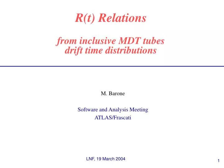
R(t) Relations from inclusive MDT tubes drift time distributions. M. Barone Software and Anal y s i s Meeting ATLAS/Frascati. Outline. Introduction Nomenclature The idea The recipe Garfield simulation Drift velocity r distribution r(t) determination Arrival time distribution

E N D
R(t) Relationsfrom inclusive MDT tubes drift time distributions M.Barone Software and Analysis Meeting ATLAS/Frascati
Outline • Introduction • Nomenclature • The idea • The recipe • Garfield simulation • Drift velocity • r distribution • r(t) determination • Arrival time distribution • R(t) relation • Data time spectrum: t0 determination • Results • Residual • Conclusions M. Barone
Nomenclature muon track • Assumption • Uniform illumination of drift tube with tracks • Definitions • Rthr = Distance traveled by the 25th ionization electron (under the assumption that the signal threshold is reached by the 25th e-) • R = Distance of minimum approach of the track to the sensing wire • r = generic distance of a point from the sensing wire • Dy = average distance of the “25th e-” origin from the point of closest approach Rthr Dy R r • Goal • Associate the arrival time of the “25th e-” to the track’s distance of minimum approach (R) determine the R(t) relation M. Barone
R(t) relation determination: the idea R(t) relation is expected to be non-linear, due to the Ar/CO2 gas mixture and to the radial electric field • Drift velocity is not constant as a function of R: v (E (R) ) • In principle the distribution of the tracks with respect to R is flat, but… • Cluster fluctuations • Charge fluctuations • -rays • Inefficiency at the borders … need to be included. • Possible method to define the R(t) relation: • We know the time distribution (from data) • We can use the simulation to determine the R distribution “correct” R distribution time spectrum from data + = R(t) relation M. Barone
R(t) relation determination: Recipe • Even though Garfield does not reproduce with adequate precision the drift velocity, it allows to determine the“correct” Rthr distribution on an event-by-event basis, independent on the gas mixture (hypothesis to be verified): • Integrating over many tracks produced in an interval R, all possible effects (d-rays, position of production of the 25th e- -Rthr, charge fluctuations, etc.) are averaged. • Recipe • Get the r(t) distribution from MC: this is the distance r at which an e- needs to be created in order to reach the sensing wire at time t. • Obtain from MC the arrival time of the 25th e- for each simulated track. • Use the r(t) function to obtain a distribution of Rthr in the MC corresponding to the previous simulated arrival times. Garfield drift velocity for a given gas mixture Garfield time spectrum + = “correct” Rthr distribution M. Barone
Garfield: gas mixture • Garfield-Magboltz used to calculate properties of three different gas-mixture: • Ar 93% , CO2 7% (standard mixture) GAS_MIX_1 • GAS_MIX_1 + 100ppm H20 GAS_MIX_2 • Ar 93.25%, CO2 6.75% + 100ppm H20 GAS_MIX_3 • Use of 100 ppm content of water vapor suggested by previous studies (ATL-COM-MUON-2003-035) M. Barone
Garfield: Drift velocity determination v(E) • Determination of the drift velocity starting from given values of the electric field E (V/cm) E field v_drift (E) Magboltz v_drift vs E cm/ms GAS_MIX_1 Does not require tracking V/cm M. Barone
Garfield: Drift velocity determination v(r) 1) Each value of E(V/cm) corresponds to a value of r (cm) Drift velocity as a function of r can be automatically determined E field r v_drift vs r v_drift (r) cm/ms GAS_MIX_2 GAS_MIX_3 cm M. Barone
Garfield: r(t) determination 2) Using the v(r) function we can calculate the drift time by integration 3) t (r) can be inverted to obtain r(t) M. Barone
Garfield: Arrival time distribution MC: GAS_MIX_2 Signal simulation: 146000 tracks t0=0 is the time given by the primary muon Signal simulation parameters: global volt= 3080global gain= 20000 global nelec = 25global thr1 = -50.E-06*nelecglobal ENC = 4200global peak = 0.23 global noisigma = ENC*peak*1.609e-7global tau=0.025 .................. convolute-signals transfer-function … (1-t/(2*tau))*(t/tau)*exp(-t/tau) The recorded time t is the arrival time of the 25th electron for each track M. Barone
Garfield: Rthr distribution Rthr distribution can be determined from the time spectrum and the r(t) relation obtained for a given gas mixture MC: GAS_MIX_2 + = M. Barone
Garfield: Rthr distribution, check Hypothesis: Rthr distributions should be the same for different gas mixture (verified simulating 14600 tracks for each gas mixture) Yes! MC: GAS_MIX_1 MC: GAS_MIX_2 MC: GAS_MIX_3 Rthr (cm) M. Barone
Test beam data: time spectrum data: run 1559 BIL2, ml1 Translate horizontally MC time spectrum to superimpose it with the data histo Register the value of the shift: t0 =585 counts Register the value of tmax: tmax = 1520 counts Garfield M. Barone
Test beam data: time spectrum tmin = 0 tmax = 925 counts M. Barone
R(t) relation determination MC DATA MC 1) Divide the Rmax-Rmin interval in 100 bins, each one containing an equal number of events Nevents(MC)/nbins= 1442.66 1) Divide the tmax-tmin interval in 100 bins, each one containing an equal number of events Nevents(data)/nbins = 1962.24 Nevents (data) = 196224 nbins = 100 max_content = Nevents/nbins =1962.24 Nevents (MC) = 144266 nbins = 100 max_content = Nevents/nbins =1442.66 2) Use the extreme of all these intervals do define Rthr values; transform Rthr into R by quadratically subtracting the average Dy (see figure on slide 3) 2) Use the extreme of all these intervals do define TDC values M. Barone
R(t) relation: result 4) The relationship between the corresponding values provide us with the R(t) relation we were looking Garfield + data Garfield M. Barone
Residuals for run 1559 M. Barone
Check 1) divide the MC sample of 146000 drift times in two independent sub-samples containing 73000 events each: MC1, MC2 2) use MC1 sample to determine Rthr distribution MC1 + = MC1 3) use MC2 sample and Rthr distribution from MC1 sample to determine r(t) relation MC2 = + MC1 M. Barone
Check 4) compare the r(t) relation with the relation obtained by Garfield using sample MC1 50 micron Garfield (MC1) + MC2 Garfield (MC1) Mean: -0.7E-02 RMS: 0.2E-01 n = 100 bins Delta r (mm) M. Barone
Conclusions • A method for the determination of R(t) relations has been proposed. • Benefits: • a lot of available statistics • R(t) relation can be determined for each tube • no dependence on the tracking method • very fast method Work in progress: use of “clean” TDC spectra analysis of more runs MC: more statistics comparison with other R(t) relations (Calib, …) Understand and quantify the limit of this method (by tracking, …) ….. M. Barone