Download
1 / 15
150 likes | 171 Views
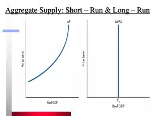
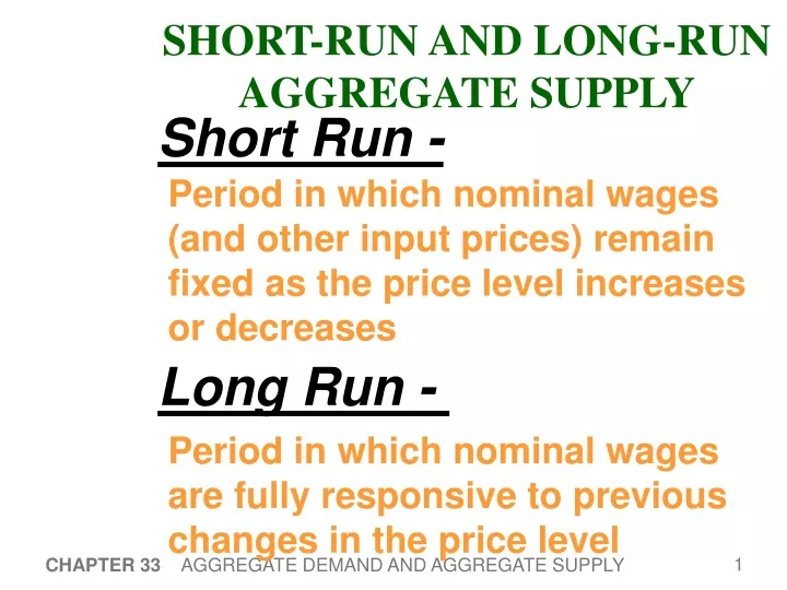
SHORT-RUN AND LONG-RUN AGGREGATE SUPPLY. Short Run -. Period in which nominal wages (and other input prices) remain fixed as the price level increases or decreases. Long Run -. Period in which nominal wages are fully responsive to previous changes in the price level.

E N D
SHORT-RUN AND LONG-RUN AGGREGATE SUPPLY Short Run - Period in which nominal wages (and other input prices) remain fixed as the price level increases or decreases Long Run - Period in which nominal wages are fully responsive to previous changes in the price level CHAPTER 33 AGGREGATE DEMAND AND AGGREGATE SUPPLY
SHORT-RUN AGGREGATE SUPPLY A higher price level increases profits and output moving the economy from a1 to a2 AS1 P2 a2 Price Level P1 a1 o Q1 Q2 Real domestic output CHAPTER 33 AGGREGATE DEMAND AND AGGREGATE SUPPLY
SHORT-RUN AGGREGATE SUPPLY A lower price level decreases profits and output moving the economy from a1 to a3 AS1 P2 a2 Price Level P1 a1 P3 a3 o Q3 Q1 Q2 Real domestic output CHAPTER 33 AGGREGATE DEMAND AND AGGREGATE SUPPLY
LONG RUN AGGREGATE SUPPLY A higher price level results in higher nominal wages and thus shifts the short-run aggregate supply to the left ASLR AS2 b1 AS1 P2 a2 a1 Price Level P1 o Q1 Q2 Real domestic output CHAPTER 33 AGGREGATE DEMAND AND AGGREGATE SUPPLY
LONG RUN AGGREGATE SUPPLY A lower price level results reduces nominal wages and shifts the short-run aggregate supply to the right ASLR AS2 b1 AS1 P2 a2 AS3 a1 Price Level P1 P3 a3 c1 o Q3 Q1 Q2 Real domestic output CHAPTER 33 AGGREGATE DEMAND AND AGGREGATE SUPPLY
LRAS1 LRAS2 P Y ’ YN Why the LRASCurve Might Shift 0 Any event that changes any of the determinants of YN will shift LRAS. Example: Immigration increases L, causing YN to rise. YN CHAPTER 33 AGGREGATE DEMAND AND AGGREGATE SUPPLY
LRAS1990 P LRAS1980 LRAS2000 P2000 P1990 AD2000 P1980 AD1990 AD1980 Y Using AD& ASto Depict LRGrowth and Inflation 0 Over the long run, tech. progress shifts LRAS to the right and growth in the money supply shifts AD to the right. Result: ongoing inflation and growth in output. Y2000 Y1980 Y1990 CHAPTER 33 AGGREGATE DEMAND AND AGGREGATE SUPPLY
Economic Fluctuations 0 • Caused by events that shift the AD and/or AS curves. • Four steps to analyzing economic fluctuations: 1.Determine whether the event shifts AD or AS. 2. Determine whether curve shifts left or right. 3. Use AD-AS diagram to see how the shift changes Y and P in the short run. 4. Use AD-AS diagram to see how economy moves from new SR eq’m to new LR eq’m. CHAPTER 33 AGGREGATE DEMAND AND AGGREGATE SUPPLY
Two Big AD Shifts: 1. The Great Depression 0 From 1929-1933, • money supply fell 28% due to problems in banking system • stock prices fell 90%, reducing C and I • Y fell 27% • P fell 22% • u-rate rose from 3% to 25% U.S. Real GDP, billions of 2000 dollars CHAPTER 33 AGGREGATE DEMAND AND AGGREGATE SUPPLY
Two Big AD Shifts: 2. The World War II Boom 0 From 1939-1944, • govt outlays rose from $9.1 billion to $91.3 billion • Y rose 90% • P rose 20% • unemp fell from 17% to 1% U.S. Real GDP, billions of 2000 dollars CHAPTER 33 AGGREGATE DEMAND AND AGGREGATE SUPPLY
LRAS P SRAS1 SRAS2 P1 P2 B AD1 P3 C AD2 Y YN Y2 The Effects of a Shift in AD 0 Event: stock market crash 1. affects C, AD curve 2. C falls, so AD shifts left 3. SR eq’m at B. P and Y lower,unemp higher 4. Over time, PE falls, SRAS shifts right,until LR eq’m at C.Y and unemp back at initial levels. A CHAPTER 33 AGGREGATE DEMAND AND AGGREGATE SUPPLY
ACTIVE LEARNING 2: Exercise 0 • Draw the AD-SRAS-LRAS diagram for the U.S. economy, starting in a long-run equilibrium. • A boom occurs in Canada. Use your diagram to determine the SR and LR effects on U.S. GDP, the price level, and unemployment. 12
LRAS P SRAS2 SRAS1 C P3 B P2 AD2 P1 AD1 Y YN Y2 ACTIVE LEARNING 2: Answers 0 Event: boom in Canada 1. affects NX, AD curve 2. shifts AD right 3. SR eq’m at point B. P and Y higher,unemp lower 4. Over time, PE rises, SRAS shifts left,until LR eq’m at C.Y and unemp back at initial levels. A 13
LRAS P SRAS2 SRAS1 B P2 P1 A AD1 Y YN Y2 The Effects of a Shift in SRAS 0 Event: oil prices rise 1. increases costs, shifts SRAS(assume LRAS constant) 2. SRAS shifts left 3. SR eq’m at point B. P higher, Y lower,unemp higher From A to B, stagflation, a period of falling output and rising prices. CHAPTER 33 AGGREGATE DEMAND AND AGGREGATE SUPPLY
LRAS P SRAS2 P3 C SRAS1 B P2 P1 A AD2 AD1 Y YN Y2 Accommodating an Adverse Shift in SRAS 0 If policymakers do nothing, 4. Low employment causes wages to fall, SRAS shifts right,until LR eq’m at A. Or, policymakers could use fiscal or monetary policy to increase AD and accommodate the AS shift: Y back to YN, butP permanently higher. CHAPTER 33 AGGREGATE DEMAND AND AGGREGATE SUPPLY