Download
1 / 7
70 likes | 86 Views
Long run aggregate Supply. Learning objectives. To be able to identify and explain the three gradients on an long run aggregate supply curve To become familiar with the components of long run aggregate supply

E N D
Learning objectives • To be able to identify and explain the three gradients on an long run aggregate supply curve • To become familiar with the components of long run aggregate supply • To appreciate the difference between the short run aggregate supply (SRAS)curve and the long run aggregate supply (LRAS)curve • To be able to distinguish between inward and outward shifts of the long run aggregate supply curve • https://www.youtube.com/watch?v=UwAQRnpVMzI
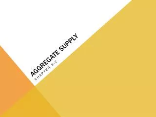
Aggregate Supply (long run, Keynesian) • The price level makes reference to the retail price index (RPI). • Real output refers to the quantity of goods and services produced in the economy. • 0A refers to the level of output where the factors of production are used to the optimum. • As output beyond 0A the factors of production become scare, this is most notable in the labour market. • The scarcity causes their price to rise thus increasing the price level. • There comes a point at which the factors of production become exhausted. This is most notable in the labour market and is known as the full employment level of output. Price level AS Real output A B Optimum Capacity output Full Capacity output 0
Combining the components of AS • Imagine a series of individual supply curves for the following:- • These are combined to produce the AS curve. Price level AS Real output
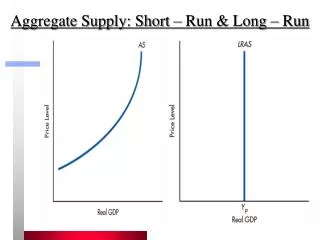
Aggregate Supply (long run) • The long run aggregate supply curve (LRAS) is vertical when all factors of production are fully employed. Price level LRAS1 Real output
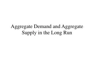
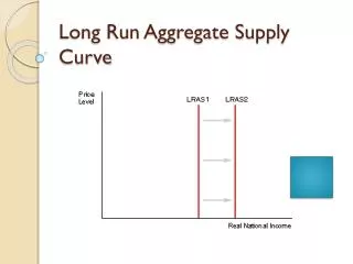
Aggregate Supply (long run, Classical) • The LRAS will shift as a there is a change in the availability of the factor of production. • Land - The discovery of new natural resources. • Labour - an increase in the working population • Capital - Improvements in technology • Entrepreneurship- Improvements in entrepreneurial culture (a more free market approach to running the economy). Price level LRAS1 LRAS2 Real output
Short run and long run aggregate supply curve • https://www.youtube.com/watch?v=WSM2U-U6u34&t=166s