Download
1 / 42
430 likes | 676 Views
Lecture 6 Sept 16 Chapter 2 continue MIPS translating c into MIPS – examples MIPS simulator (MARS and SPIM). Finding the Maximum in an array. Array A is stored in memory beginning at the address given in $s1. Array length is given in $s2.

E N D
Lecture 6 Sept 16 • Chapter 2 • continue MIPS • translating c into MIPS – examples • MIPS simulator (MARS and SPIM)
Finding the Maximum in an array Array A is stored in memory beginning at the address given in $s1. Array length is given in $s2. Find the largest integer in the list and copy it into $t0. Solution Scan the list, holding the largest element identified thus far in $t0.
Finding the Maximum in an array lw $t0,0($s1) # initialize maximum to A[0] addi $t1,$zero,0 # initialize index i to 0 loop: add $t1,$t1,1 # increment index i by 1 beq $t1,$s2,done # if all elements examined, quit sll $t2,$t2,2 # compute 4i in $t2 add $t2,$t2,$s1 # form address of A[i] in $t2 lw $t3,0($t2) # load value of A[i] into $t3 slt $t4,$t0,$t3 # maximum < A[i]? beq $t4,$zero,loop # if not, repeat with no change addi $t0,$t3,0 # if so, A[i] is the new maximum j loop # change completed; now repeat done: # continuation of the program
SPIM – A simulator for MIPS Assembly language • Home page of SPIM: • http://www.cs.wisc.edu/~larus/spim.html • A useful document: • http://www.cs.wisc.edu/HP_AppA.pdf
Tutorials on SPIM There are many good tutorials on SPIM. Here are two introductory ones: http://www.cs.umd.edu/class/fall2001/cmsc411/projects/spim/ http://users.ece.gatech.edu/~sudha/2030/temp/spim/spim-tutorial.html Please read (watch) them once and refer to them when you need help.
SPIM simulator – how to run? We will implement the code written earlier (finding the max element in an array) using the SPIM simulator. Code is shown below:
Creating the code and the text segments in SPIM • .text • .globl __start • __start: • la $s1, array # initialize array • lw $t0, ($s1) • la $t6, count • lw $s2, ($t6) • la is a pseudo-instruction (load address). • We use this to input the starting address and the size of the array into registers $s1 and $t6.
Include the code to be executed addi $t1,$zero, 0 # initialize index i to 0 loop: add $t1,$t1,1 # increment index i by 1 beq $t1,$s2,done # if all elements examined, quit add $t2,$t1,$t1 # compute 2i in $t2 add $t2,$t2,$t2 # compute 4i in $t2 add $t2,$t2,$s1 # form address of A[i] in $t2 lw $t3,0($t2) # load value of A[i] into $t3 slt $t4,$t0,$t3 # maximum < A[i]? beq $t4,$zero,loop # if not, repeat with no change addi $t0,$t3,0 # if so, A[i] is the new maximum j loop # change completed; now repeat done:
Input to the program – Data Segment .data array: .word 3,4,2,6,12,7,18,26,2,14,19,7,8,12,13 count: .word 15 endl: .asciiz "\n" ans2: .asciiz "\nmax = "
Output the result Input array: 3,4,2,6,12,7,18,26,2,14,19,7,8,12,13
System calls for output la $a0,ans2 li $v0,4 syscall # print "\nmax = " move $a0,$t0 li $v0,1 syscall # print max la $a0,endl # system call to print li $v0,4 # out a newline syscall li $v0,10 syscall # end
Procedure Calling Steps required • Place parameters (arguments) in registers • Transfer control to procedure • Acquire storage for procedure • Perform procedure’s operations • Place result in register for caller • Return to place of call §2.8 Supporting Procedures in Computer Hardware
Register Usage • $a0 – $a3: arguments (reg’s 4 – 7) • $v0, $v1: result values (reg’s 2 and 3) • $t0 – $t9: temporaries • Can be overwritten by callee • $s0 – $s7: saved • Must be saved/restored by callee • $gp: global pointer for static data (reg 28) • $sp: stack pointer (reg 29) • $fp: frame pointer (reg 30) • $ra: return address (reg 31)
Procedure Call Instructions • Procedure call: jump and link jal ProcedureLabel • Address of following instruction put in $ra • Jumps to target address • Procedure return: jump register jr $ra • Copies $ra to program counter • Can also be used for computed jumps • e.g., for case/switch statements
Leaf Procedure Example • c code: int leaf_example (int g, h, i, j){ int f; f = (g + h) - (i + j); return f;} • Arguments g, …, j in $a0, …, $a3 • f in $s0 (hence, need to save $s0 on stack) • Result in $v0
Leaf Procedure Example • MIPS code: leaf_example: addi $sp, $sp, -4 sw $s0, 0($sp) add $t0, $a0, $a1 add $t1, $a2, $a3 sub $s0, $t0, $t1 add $v0, $s0, $zero lw $s0, 0($sp) addi $sp, $sp, 4 jr $ra Save $s0 on stack Procedure body Result Restore $s0 Return
Non-Leaf Procedures • Procedures that call other procedures are known as non-leaf procedures. • For nested call, caller needs to save on the stack: • Its return address • Any arguments and temporaries needed after the call • Restore from the stack after the call
Non-Leaf Procedure Example • C code: int fact (int n){ if (n < 1) return f; else return n * fact(n-1);} • Argument n in $a0 • Result in $v0
Non-Leaf Procedure Example MIPS code: fact: addi $sp, $sp, -8 # adjust stack for 2 items sw $ra, 4($sp) # save return address sw $a0, 0($sp) # save argument slti $t0, $a0, 1 # test for n < 1 beq $t0, $zero, L1 addi $v0, $zero, 1 # if so, result is 1 addi $sp, $sp, 8 # pop 2 items from stack jr $ra # and returnL1: addi $a0, $a0, -1 # else decrement n jal fact # recursive call lw $a0, 0($sp) # restore original n lw $ra, 4($sp) # and return address addi $sp, $sp, 8 # pop 2 items from stack mul $v0, $a0, $v0 # multiply to get result jr $ra # and return
As we saw in the previous slide, the program correctly computes 12! As 12! = 479001600. But when tried for n = 13, the output is: 1932053504 This is clearly wrong! What happened? How to fix the program?
Local Data on the Stack • Local data allocated by callee • e.g., C automatic variables • Procedure frame (activation record) • Used by some compilers to manage stack storage
Memory Layout • Text: program code • Static data: global variables • e.g., static variables in C, constant arrays and strings • $gp initialized to address allowing ±offsets into this segment • Dynamic data: heap • E.g., malloc in C, new in Java • Stack: automatic storage
Character Data • Byte-encoded character sets • ASCII: 128 characters • 95 graphic, 33 control • Latin-1: 256 characters • ASCII, +96 more graphic characters • Unicode: 32-bit character set • Used in Java, C++ wide characters, … • Most of the world’s alphabets, plus symbols • UTF-8, UTF-16: variable-length encodings §2.9 Communicating with People
Byte/Halfword Operations • Could use bitwise operations • MIPS byte/halfword load/store • String processing is a common case lb rt, offset(rs) lh rt, offset(rs) • Sign extend to 32 bits in rt lbu rt, offset(rs) lhu rt, offset(rs) • Zero extend to 32 bits in rt sb rt, offset(rs) sh rt, offset(rs) • Store just rightmost byte/halfword
Target Addressing Example • Loop code from earlier example • Assume Loop at location 80000
Translation and Startup Many compilers produce object modules directly §2.12 Translating and Starting a Program Static linking
Assembler Pseudoinstructions • Most assembler instructions represent machine instructions one-to-one • Pseudoinstructions: not supported in instruction set, but assembler translates into equivalent move $t0, $t1→add $t0, $zero, $t1 blt $t0, $t1, L→slt $at, $t0, $t1bne $at, $zero, L • $at (register 1): assembler temporary
Producing an Object Module • Assembler (or compiler) translates program into machine instructions • Provides information for building a complete program from the pieces • Header: described contents of object module • Text segment: translated instructions • Static data segment: data allocated for the life of the program • Relocation info: for contents that depend on absolute location of loaded program • Symbol table: global definitions and external refs • Debug info: for associating with source code
Linking Object Modules • Produces an executable image 1. Merges segments 2. Resolve labels (determine their addresses) 3. Patch location-dependent and external refs
Loading a Program • Load from image file on disk into memory 1. Read header to determine segment sizes 2. Create virtual address space 3. Copy text and initialized data into memory • Or set page table entries so they can be faulted in 4. Set up arguments on stack 5. Initialize registers (including $sp, $fp, $gp) 6. Jump to startup routine • Copies arguments to $a0, … and calls main • When main returns, do exit syscall
Dynamic Linking • Only link/load library procedure when it is called • Requires procedure code to be relocatable • Avoids image bloat caused by static linking of all (transitively) referenced libraries • Automatically picks up new library versions
ARM & MIPS Similarities • ARM: the most popular embedded core • Similar basic set of instructions to MIPS §2.16 Real Stuff: ARM Instructions
Compare and Branch in ARM • Uses condition codes for result of an arithmetic/logical instruction • Negative, zero, carry, overflow • Compare instructions to set condition codes without keeping the result • Each instruction can be conditional • Top 4 bits of instruction word: condition value • Can avoid branches over single instructions
Fallacies • Powerful instruction higher performance • Fewer instructions required • But complex instructions are hard to implement • May slow down all instructions, including simple ones • Compilers are good at making fast code from simple instructions • Use assembly code for high performance • But modern compilers are better at dealing with modern processors • More lines of code more errors and less productivity §2.18 Fallacies and Pitfalls
Concluding Remarks • Design principles 1. Simplicity favors regularity 2. Smaller is faster 3. Make the common case fast 4. Good design demands good compromises • Layers of software/hardware • Compiler, assembler, hardware • MIPS: typical of RISC ISAs §2.19 Concluding Remarks
Concluding Remarks • Measure MIPS instruction executions in benchmark programs • Consider making the common case fast • Consider compromises