Download
1 / 15
170 likes | 185 Views
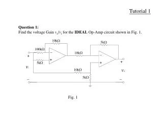
Tutorial 1. CUFSM 3.12. Default Cee section in bending Objective To introduce the conventional finite strip method and gain a rudimentary understanding of how to perform an analysis and interpret the results. A the end of the tutorial you should be able to enter simple geometry

E N D
Tutorial 1 CUFSM3.12 • Default Cee section in bending • Objective To introduce the conventional finite strip method and gain a rudimentary understanding of how to perform an analysis and interpret the results. • A the end of the tutorial you should be able to • enter simple geometry • enter loads (stresses) • perform a finite strip analysis • manipulate the post-processor
3. SELECT Cross-section geometry is entered by filling out the nodes and the elements, e.g., node 6 is at coordinate 0.0,6.0 **separate your entries by single spaces** We will discuss more about all those 1’s after the nodal coordinates and the last column in the Nodes section later on. You can always press the ‘?’ buttons if you want to learn more now. Let’s take a look at the elements. (follow the arrows) 1. UNCHECK 2. CHECK
3. SELECT Elements define how the geometry is connected, how thick the member is, and what material a particular element is composed of. For example element 5, connects nodes 5 and 6 together, has a thickness of 0.1 in. and uses material “100” - material 100 is defined above in the Material Properties Section. Let’s take a look at the loading. (follow the arrows) 1. UNCHECK 2. CHECK
3. SELECT Each node has a “stress” assigned to it. Our analysis will give a “buckling load factor” that is a multiplier times the inputted stresses. In this case the stresses amount to a pure bending case with fy=50 ksi. Let’s take a look at the stress distribution. (follow the arrows) 1. UNCHECK 2. CHECK
1 2 select 1, analysis will proceed, then will go to 2 automatically. The stress distribution (the loading) is clearly shown to be pure bending. Note the “Lengths” below. These are the half-wavelengths that we will analyze. Each half-wavelength has a different buckling load factor. Let’s Analyze and then go to the Post processor to view the results.
This screen shows what “Post” looks like after you analyze. The buckling mode for the red circle point is shown above. Select different half-wavelengths using the arrow buttons above and plot the different mode shapes. The minima of the buckling curve below identify important locations to examine. 2 select 1, 4 times, until the red circle below moves to 5.0, then select 2, to view the buckling mode 1 “red circle”= where you are at
The local buckling mode is shown to the left. The mode repeats at a half-wavelength of 5.0 in. (See summary above plot and numbers below in the buckling curve). The buckling load factor is 1.03 for local buckling. This means elastic critical local buckling occurs at 1.03 times the stress distribution entered - remember the stress magnitudes from before? 2 select 1, until the red circle moves to 40.0, then select 2, to view the distortional buckling mode 1 note, the scale of the buckling mode is arbitrary! 1 or -1 are equally valid, as is 0.5 or 4, or any other convenient multiplier.
3 The distortional buckling mode is shown to the left. The mode repeats at a half-wavelength of 40.0 in. The buckling load factor is 0.82. This means elastic critical distortional buckling occurs at 0.82 times the stress distribution entered. follow 1,2,3 to take a look at the buckling modes in 3D 1 2
2 this is distortional buckling, select 1 and go back to 5.0, then select 2, let’s look at local buckling first One can use ‘Z’ to zoom out or in and ‘R’ to ratate. 1
The 3D plot to the left shows local buckling at a half-wavelength of 5.0 in. Note, the 2D plot presented earlier shows the maximum cross-section deflected shape only. CUFSM finite strip analysis assumes a single half sine wave in the longitudinal direction (as shown). Return to a half-wavelength of 40 in. to see the distortional buckling mode. The lengths that are analyzed in the plot below are selected by the user. Let’s add some points in the circled sections below to smooth out our plot. Select input.
2 3 select 2, analysis will proceed, then will go to 3 automatically 1. Add the additional “lengths below”. All the half-wavelengths that are entered below are analyzed. If you are only concerned about a particular range of half-wavelength (e.g., local buckling) then you may remove some lengths.
Q: What would happen if I assumed the member always buckled in two half sine waves (i.e a full sine wave) instead of one? A: You would see the same buckling curve, but it would be translated to the right. For example - local buckling has a minimum at 5.0 in. for one half sine wave, and will have a minimum at (2)(5.0) = 10.0 in. for two half sine waves. The analysis results for all of the lengths are shown below. Q: Why is the load factor at a half-wavelength of 10 in. greater than at 5.0 in? A: Because the analysis always assumes buckling is in a single half sine wave, this may not be how the actual member buckles. See next slide for result
(2) This is a specially constructed curve, in which two half sine waves have been assumed throughout the analysis of the Cee in bending. Note now that local occurs at (2)(5.0) = 10.0 in., and distortional at (2)(40.0) = 80.0 in. In a real structure the buckling mode is free to form any number of half sine waves - therefore only the minimums of the first curve are of primary interest. (1) This is the same buckling curve we have been looking at for the Cee in bending. Note the familiar minimums: local at 5.0 in., and distortional at 40.0 in. This curve, like all other finite strip analysis generated by CUFSM assumes a single half sine wave in the longitudinal direction. You can choose which one to show. Q: What would 3 half sine waves look like? 4?
Tutorial 1: Conclusions CUFSM3.12 • Default Cee section in bending • Objective To introduce the conventional finite strip method and gain a rudimentary understanding of how to perform an analysis and interpret the results. • A the end of the tutorial you should be able to • enter simple geometry • enter loads (stresses) • perform a finite strip analysis • manipulate the post-processor