Geometric Correction of Imagery

1. Geometric Correction of Imagery Lecture 4 prepared by R. Lathrop 10/99 updated 10/03 Readings: ERDAS Field Guide 6th Ed. Ch 9, 12 App B Map Projections

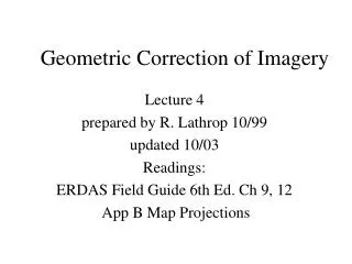
2. Geometric Correction of Imagery • The intent is to compensate for the distortions introduced by a variety of factors, so that corrected imagery will have the geometric integrity of a planimetric map • Systematic distortions: predictable; corrected by mathematical formulas. These often corrected during preprocessing • Nonsystematic or random distortions: corrected statistically by comparing with ground control points. Often done by end-user

3. Registration vs. Rectification • Registration: reference one image to another of like geometry (I.e. same scale) • Rectification: process by which the geometry of an image area is made planimetric by referencing to some standard map projection • Reprojection: transformation from one projection system to another using a standard series of mathematical formulas

4. Rectification • Whenever accurate area, direction and distance measurements are required, rectification is required. • Integration of the image to a GIS: need to be able to georeference an individual’s pixel location to its true location on the Earth’s surface. • Standard map projections: Lat/long, UTM, State Plane

5. Map Projections • The manner in which the spherical (3d) surface of the Earth is represented on a flat (2-d) surface. • Think about lighting up the interior of a transparent globe that has lines and features boundaries drawn on its surface. If the lighted globe is placed near a blank wall, you can see the shadow of the globe’s map on the wall. You will have “projected” a 3d surface to a 2d surface. • All projections involve some form of distortion

6. Properties of Map Projections • Conformality: preserves shape of small areas • Equivalence: preserves areas, not shape • Equidistance: scale of distance constant • True direction: preserves directions, angles • There is no single “perfect” map projection, all projections require some form of compromise

7. Families of Map Projections • Cylindrical • Conical • Azimuthal Distortion is minimized along the line of contact • Tangent: intersect along one line • Secant: intersects along two lines Graphic from www.pobonline.com

8. Types of Coordinates • Geographical: spherical coordinates based on the network of latitude and longitude lines, measured in degrees • Planar: Cartesian coordinates defined by a row and column position on a planar (X,Y) grid, measured in meters or feet. Examples include: Universal Transverse Mercator (UTM) and State Plane

9. Latitude and Longitude Coordinates Spherical coordinates are based on the network of latitude (N-S) and longitude lines (E-W), measured in angular degrees Latitude lines or parallels Longitude lines or meridians Graphics from: http://www-istp.gsfc.nasa.gov/stargaze/Slatlong.htm

10. Universal Transverse Mercator (UTM) UTM is a planar coordinate system Globe subdivided into 60 zones - 6o longitude wide Referenced as Eastings & Northings, measured in meters Graphics from: http://mac.usgs.gov/mac/isb/pubs/factsheets/fs07701.html

11. State Plane Coordinate system State Plane is a planar-rectangular coordinate system Each state has its own coordinate system oriented to the particular shape of the state. SP based on a conformal map projection. Referenced as X & Y coordinates, measured in feet Graphics from : www.pobonline.com/CDA/Article_Information/GPS_Index/1,2459,,00.html

12. Factors in Choosing a Map Projection • Type of map • Size and configuration of area to be mapped • Location of map on globe: tropics, temperate or polar regions • Special properties that must be preserved • Types of data to be mapped • Map accuracy • Scale

13. Other Considerations • Spheroid: the sphere isn’t a true sphere. Most projections require the definition of a spheroid (or ellipsoid), which is a model of the earth’s shape. Choose the spheroid appropriate for your geographic region. • Datum: reference elevation, determined by National Geodetic Survey

14. Coordinate Transformations • Both registration and rectification require some form of coordinate transformation • Transformation equation allows the reference coordinates for any data file location to be precisely estimated; to transform from one coordinate space to another

15. Transforming from one Coordinate System to Another x,y : map X’, Y’ : image Map Image

16. Transformation Equation • To transform from the data file coordinates to a reference coordinate system requires a change in: • Scale • Rotation • Translation

17. Example: Transformation Equationfrom Jensen 1996 p 133 X’ = -382.08 + 0.034187x - 0.005481y Y’ = 130162 - 0.005576x - 0.0349150y x,y : map X’, Y’ : image

18. Example: Transformation Equationfrom Jensen 1996 p 133 X’ = -382.08 + 0.034187x - 0.005481y Y’ = 130162 - 0.005576x - 0.0349150y x,y : map X’, Y’ : image Given an x, y location, compute the X’, Y’ location. x = 598,285 E y = 3,627,280 N X’ = -382.08 + 20453.5 - 19881.1 = 190.3 Y’ = 130162 - 3336.0 - 126646.5 = 180

19. Calculating Transformation Equations • The statistical technique of least squares regression is generally used to determine the coefficients for the coordinate transformation equations. • Want to minimize the residual error (RMS error) between the predicted (X’) and observed (X’orig) locations • RMS error = SQRT[(X’ - X’orig)2 + (Y’ - Y’orig)2]

20. Ground Control Points (GCP) • Ground control points (GCPs): locations that are found both in the image and in the map • The GCP coordinates are recorded from the map and from the image and then used in the least squares regression analysis to determine the coordinate transformation equations • Want to use features that are readily identifiable and not likely to move, e.g., road intersections

21. y Y’ x X’ Ground Control Points (GCP) Map Image

22. 1st order transformation • Also referred to as an affine transformation • X’ = ao + a1x + a2y X’,Y’ = image Y’ = bo + b1x + b2y x, y = map • ao, bo: for translation • a1, b1: for rotation and scaling in x direction • a2, b2: for rotation and scaling in y direction • 6 unknowns, need minimum of 3 GCP’s • difference in scale in X & Y, true shape not maintained but parallel lines remain parallel

23. 2nd order polynomial • X’ = ao + a1x + a2y + a3x2+ a4y2 + a5xy Y’ = bo + b1x + b2y + b3x2+ b4y2 + b5xy • 12 unknowns, need minimum of 6 GCP’s • nonlinear differences in scale in X & Y, true shape not maintained, parallel lines no longer remain parallel • Higher order polynomials also known as rubber sheeting

24. Minimum of GCP’s Higher orders of transformation can be used to correct more complicated types of distortion. However, to use a higher order of transformation, more GCP’s are needed. The minimum number of GCP’s required to perform a transformation of order t equals: ( ( t + 1 ) ( t + 2 ) ) 2 t Order Min. # of GCP’s 1 3 2 6 3 10 4 15

25. Ortho-rectification • Orthorectification: correction of the image for topographic distortion. This is especially important in mountainous areas where there can be distortions (e.g. scale changes) due to the varying elevations in the image scene. • Corrected by including Z values (elevation from a DEM) and photogrammetric principles

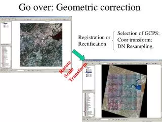
26. Rectification Process • Locate ground control points • Compute and test a coordinate transformation matrix. Iterative process till required RMS error tolerance is reached. • Create an output image in the new coordinate system. The pixels must be resampled to conform to the new grid.

27. Root Mean Square (RMS) Error RMS Error per GCP, Ri: Ri = SQRT( XRi2 + YRi2) where Ri = RMS Error per GCPi XRi = X residual for GCPi YRi = Y residual for GCPi Source GCP X residual RMS error Y residual Retransformed GCP

28. Total RMS Error X RMS error, Rx Y RMS error, Ry Rx = SQRT( 1/n (SUM XRi2)) Ry = SQRT( 1/n (SUM YRi2)) where XRi = X residual for GCPi YRi = Y residual for GCPi n = # of GCPs Total RMS, T = SQRT(Rx2 +Ry2) Error Contribution by Individual GCP, Ei : Ei = Ri / T

29. RMS Error: Example X Y xi xr Resid Resid2 yi yr Resid Resid2 228.0 228.5 0.5 0.25 242.0 241.3 -0.7 0.49 152.0 151.5 -0.5 0.25 237.0 237.0 0.0 0.0 199.0 199.2 0.2 0.04 318.0 317.4 -0.6 0.36 174.0 173.8 -0.2 0.04 352.0 352.1 0.1 0.01 42.0 41.9 -0.1 0.01 430.0 435.5 0.5 0.25 TotalSum 0.59 1.11 X RMS Error = RMSx = SQRT(0.59/5) = SQRT(0.118) = 0.34 Y RMS Error = RMSy = SQRT(1.11/5) = SQRT(0.222) = 0.47 Total RMS Error = SQRT(0.118 + 0.222) = SQRT(0.340) = 0.58

30. RMS Error: Example Error Contribution per GCP RxRyRi Ei GCP1 0.25 0.49 0.86 1.48 GCP2 0.25 0.0 0.50 0.86 GCP3 0.04 0.36 0.64 1.10 GCP4 0.04 0.01 0.22 0.38 GCP5 0.01 0.25 0.51 0.88 where Ri = RMS Error per GCP Ei =Error Contribution by Individual GCPi

31. RMS Error Tolerance • Rectification always entails some amount of error. The amount of error that the user is willing to tolerate depends on the application. • RMS error is thought of as a error tolerance radius or window. The re-transformed pixel is within the window formed by the source pixel and a radius buffer • For example: a RMS of 0.5 pixel would still put the transformed coordinate within the source pixel

32. 2 pixel RMS error tolerance (radius) Source pixel Retransformed coordinates within this range are considered correct RMS Error Tolerance From ERDAS Imagine Field Guide 5th ed.

33. Error tolerance Either as CE 90% or linear RMSE Mapped pixel vs. “true” ground location The greater the geometric accuracy the higher the cost Geometric Accuracy: how close do you need? Example from Quickbird Scale CE90% RMSE 1:50,000 25.5m 15.4m 1:5,000 4.2m 2.6M http://www.digitalglobe.com/product/ortho_imagery.shtml

34. Resampling process • The rectification/resampling process at first glance appears to operate backwards in that the transformation equation goes from the map to the image, when you might expect it to go from the image to the map. • The process works as follows: - create output grid - backtransform from map to image - resample to fill output grid

35. Resampling: for each output pixel calculate the closest input coordinate Rectified Output image Original Input image Map Image

36. Resampling process • An empty output matrix is created in the map coordinate systems at the desired starting coordinate location and pixel size • Using the transformation equation, the coordinates of each pixel in the output map matrix are transformed to determine their corresponding location in the original input image • This transformed cell location will not directly overlay a pixel in the input matrix. Resampling is used to assign a DN value to the output matrix pixel - determined on the basis of the pixel values which surround its transformed position in the original input image matrix

37. Resampling Methods • Nearest-neighbor • Bilinear Interpolation • Cubic Convolution

38. Nearest-neighbor • Substitutes in DN value of closest pixel. Transfers original pixel brightness values without averaging them. Keeps extremes. • Suitable for use before classification • Fastest to compute • Results in blocky “stair stepped” diagonal lines

39. Nearest neighbor resampling: chose closest single pixel Rectified Output image Original Input image Map Image

40. Bilinear Interpolation • Distance weighted average of the DN’s of the four closest pixels • More spatially accurate than nearest neighbor; smoother, less blocky • Still fast to compute • Pixel DN’s are averaged, smoothing edges and extreme values

41. Bilinear Interpolation: weighted average of four closest pixels Rectified Output image Original Input image Map Image

42. Cubic Convolution • Evaluates block of 16 nearest pixels, not strictly linear interpolation • Mean and variance of output distribution match input distribution, however data values may be altered • Can both sharpen image and smooth out noise • Computationally intensive

43. Cubic Convolution: weighted average of 16 closest pixels Rectified Output image Original Input image Map Image