Download
1 / 38
680 likes | 1.22k Views
Geometric Correction. Lecture 5 Feb 18, 2005. 1. What and why.

E N D
Geometric Correction Lecture 5 Feb 18, 2005
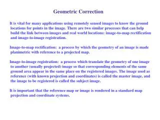
1. What and why • Remotely sensed imagery typically exhibits internal and externalgeometricerror. It is important to recognize the source of the internal and external error and whether it is systematic(predictable)ornonsystematic(random). Systematic geometric error is generally easier to identify and correct than random geometric error • It is usually necessary to preprocess remotely sensed data and remove geometric distortion so that individual picture elements (pixels) are in their proper planimetric (x, y) map locations. • This allows remote sensing–derived information to be related to other thematic information in geographic information systems (GIS) or spatial decision support systems (SDSS). • Geometrically corrected imagery can be used to extract accurate distance, polygon area, and direction (bearing) information.
Internal geometric errors • Internal geometric errors are introduced by the remote sensing system itself or in combination with Earth rotation or curvature characteristics. These distortions are often systematic (predictable) and may be identified and corrected using pre-launch or in-flight platform ephemeris (i.e., information about the geometric characteristics of the sensor system and the Earth at the time of data acquisition). These distortions in imagery that can sometimes be corrected through analysis of sensor characteristics and ephemeris data include: • skew caused by Earth rotation effects, • scanning system–induced variation in ground resolution cell size, • scanning system one-dimensional relief displacement, and • scanning system tangential scale distortion.
External geometric errors • External geometric errors are usually introduced by phenomena that vary in nature through space and time. The most important external variables that can cause geometric error in remote sensor data are random movements by the aircraft (or spacecraft) at the exact time of data collection, which usually involve: • altitude changes, and/or • attitude changes (roll, pitch, and yaw).
Altitude Changes • Remote sensing systems flown at a constant altitude above ground level (AGL) result in imagery with a uniform scale all along the flightline. For example, a camera with a 12-in. focal length lens flown at 20,000 ft. AGL will yield 1:20,000-scale imagery. If the aircraft or spacecraft gradually changes its altitude along a flightline, then the scale of the imagery will change. Increasing the altitude will result in smaller-scale imagery (e.g., 1:25,000-scale). Decreasing the altitude of the sensor system will result in larger-scale imagery (e.g, 1:15,000). The same relationship holds true for digital remote sensing systems collecting imagery on a pixel by pixel basis.
Attitude changes • Satellite platforms are usually stable because they are not buffeted by atmospheric turbulence or wind. Conversely, suborbital aircraft must constantly contend with atmospheric updrafts, downdrafts, head-winds, tail-winds, and cross-winds when collecting remote sensor data. Even when the remote sensing platform maintains a constant altitude AGL, it may rotate randomly about three separate axes that are commonly referred to as roll, pitch, and yaw. • Quality remote sensing systems often have gyro-stabilization equipment that isolates the sensor system from the roll and pitch movements of the aircraft. Systems without stabilization equipment introduce some geometric error into the remote sensing dataset through variations in roll, pitch, and yaw that can only be corrected using ground control points.
2. Conceptions of geometric correction • Geocoding: geographical referencing • Registration: geographically or nongeographically (no coordination system) • Image to Map (or Ground Geocorrection) The correction of digital images to ground coordinates using ground control points collected from maps (Topographic map, DLG) or ground GPS points. • Image to Image Geocorrection Image to Image correction involves matching the coordinate systems or column and row systems of two digital images with one image acting as a reference image and the other as the image to be rectified. • Spatial interpolation: from input position to output position or coordinates. • RST (rotation, scale, and transformation), Polynomial, Triangulation • Root Mean Square Error (RMS):The RMS is the error term used to determine the accuracy of the transformation from one system to another. It is the difference between the desired output coordinate for a GCP and the actual. • Intensity (or pixel value) interpolation (also called resampling): The process of extrapolating data values to a new grid, and is the step in rectifying an image that calculates pixel values for the rectified grid from the original data grid. • Nearest neighbor, Bilinear, Cubic
Ground control point • Geometric distortions introduced by sensor system attitude (roll, pitch, and yaw) and/or altitude changes can be corrected using ground control points and appropriate mathematical models. A ground control point(GCP) is a location on the surface of the Earth (e.g., a road intersection) that can be identified on the imagery and located accurately on a map. The image analyst must be able to obtain two distinct sets of coordinates associated with each GCP: • image coordinates specified in irows and j columns, and • map coordinates (e.g., x, y measured in degrees of latitude and longitude, feet in a state plane coordinate system, or meters in a Universal Transverse Mercator projection). • The paired coordinates (i, j and x, y) from many GCPs (e.g., 20) can be modeled to derive geometric transformation coefficients. These coefficients may be used to geometrically rectify the remote sensor data to a standard datum and map projection.
2.1 a) U.S. Geological Survey 7.5-minute 1:24,000-scale topographic map of Charleston, SC, with three ground control points identified (13, 14, and 16). The GCP map coordinates are measured in meters easting (x) and northing (y) in a Universal Transverse Mercator projection. b) Unrectified 11/09/82 Landsat TM band 4 image with the three ground control points identified. The image GCP coordinates are measured in rows and columns.
2.2 Image to image • Manuel select GCPs (the same as Image to Map) • Automatic algorithms • Algorithms that directly use image pixel values; • Algorithms that operate in the frequency domain (e.g., the fast Fourier transform (FFT) based approach used); see paper Xie et al. 2003 • Algorithms that use low-level features such as edges and corners; and • Algorithms that use high-level features such as identified objects, or relations between features.
FFT-based automatic image to image registration • Translation, rotation and scale in spatial domain have counterparts in the frequency domain. • After FFT transform, the phase difference in frequency domain will be directly related to their shifts in the space domain. So we get shifts. • Furthermore, both rotation and scaling can be represented as shifts by Converting from rectangular coordination to log-polar coordination. So we can also get the rotation and scale.
The Main IDL Codes Xie et al. 2003
ENVI Main Menus We added these new submenus Main Menu of ENVI
This is the new interface for automatic image registration TM Band 7 July 12, 1997 UTM, Zone 13N TM band 7 June 26, 1991 State Plane, TX Center 4203
Registered Image TM band 7 June 26, 1991 UTM, Zone 13N TM Band 7 July 12, 1997 UTM, Zone 13N
2.3 Spatial Interpolation • RST (rotation, scale, and transformation or shift) good for image no local geometric distortion, all areas of the image have the same rotation, scale, and shift. The FFT-based method presented early belongs to this type. If there is local distortion, polynomial and triangulation are needed. • Polynomial equations be fit to the GCP data using least-squares criteria to model the corrections directly in the image domain without explicitly identifying the source of the distortion. Depending on the distortion in the imagery, the number of GCPs used, and the degree of topographic relief displacement in the area, higher-order polynomial equations may be required to geometrically correct the data. The order of the rectification is simply the highest exponent used in the polynomial. • Triangulation constructs a Delaunay triangulation of a planar set of points. Delaunay triangulations are very useful for the interpolation, analysis, and visual display of irregularly-gridded data. In most applications, after the irregularly gridded data points have been triangulated, the function TRIGRID is invoked to interpolate surface values to a regular grid. Since Delaunay triangulations have the property that the circumcircle of any triangle in the triangulation contains no other vertices in its interior, interpolated values are only computed from nearby points.
Concept of how different-order transformations fit a hypothetical surface illustrated in cross-section. One dimension: a) Original observations. b) First-order linear transformation fits a plane to the data. c) Second-order quadratic fit. d) Third-order cubic fit.
Polynomial interpolation for image (2D) • This type of transformation can model six kinds of distortion in the remote sensor data, including: • translation in xandy, • scale changes in xandy, • rotation, and • skew. • When all six operations are combined into a single expression it becomes: • where xand y are positions in the output-rectified image or map, and x and y represent corresponding positions in the original input image.
a) The logic of filling a rectified output matrix with values from an unrectified input image matrix using input-to-output (forward) mapping logic. b) The logic of filling a rectified output matrix with values from an unrectified input image matrix using output-to-input (inverse) mapping logic and nearest-neighbor resampling. Output-to-input inverse mapping logic is the preferred methodology because it results in a rectified output matrix with values at every pixel location.
The goal is to fill a matrix that is in a standard map projection with the appropriate values from a non-planimetric image.
root-mean-square error • Using the six coordinate transform coefficients that model distortions in the original scene, it is possible to use the output-to-input (inverse) mapping logic to transfer (relocate) pixel values from the original distorted image x, y to the grid of the rectified output image, x, y. However, before applying the coefficients to create the rectified output image, it is important to determine how well the six coefficients derived from the least-squares regression of the initial GCPs account for the geometric distortion in the input image. The method used most often involves the computation of the root-mean-square error (RMS error) for each of the ground control points. where: xorigand yorigare the originalrow and column coordinates of the GCP in the image and x’and y’are the computed or estimated coordinates in the original image when we utilize the six coefficients. Basically, the closer these paired values are to one another, the more accurate the algorithm (and its coefficients).
Cont’ • There is an iterative process that takes place. First, all of the original GCPs (e.g., 20 GCPs) are used to compute an initial set of six coefficients and constants. The root mean squared error (RMSE) associated with each of these initial 20 GCPs is computed and summed. Then, the individual GCPs that contributed the greatest amount of error are determined and deleted. After the first iteration, this might only leave 16 of 20 GCPs. A new set of coefficients is then computed using the16 GCPs. The process continues until the RMSE reaches a user-specified threshold (e.g., <1 pixel error in the x-direction and <1 pixel error in the y-direction). The goal is to remove the GCPs that introduce the most error into the multiple-regression coefficient computation. When the acceptable threshold is reached, the final coefficients and constants are used to rectify the input image to an output image in a standard map projection as previously discussed.
2.4 Pixel value interpolation • Intensity (pixel value) interpolation involves the extraction of a pixel value from an x, y location in the original (distorted) input image and its relocation to the appropriate x, ycoordinate location in the rectified output image. This pixel-filling logic is used to produce the output image line by line, column by column. Most of the time the x and y coordinates to be sampled in the input image are floating point numbers (i.e., they are not integers). For example, in the Figure we see that pixel 5, 4 (x, y) in the output image is to be filled with the value from coordinates 2.4, 2.7 (x, y) in the original input image. When this occurs, there are several methods of pixel value interpolation that can be applied, including: • nearest neighbor, • bilinear interpolation, and • cubic convolution. • The practice is commonly referred to as resampling.
Nearest Neighbor The Pixel value closest to the predicted x’,y’coordinate is assigned to the output x, y coordinate.
R.D.Ramsey • ADVANTAGES: • Output values are the original input values. Other methods of resampling tend to average surrounding values. This may be an important consideration when discriminating between vegetation types or locating boundaries. • Since original data are retained, this method is recommended before classification. • Easy to compute and therefore fastest to use. • DISADVANTAGES: • Produces a choppy, "stair-stepped" effect. The image has a rough appearance relative to the original unrectified data. • Data values may be lost, while other values may be duplicated. Figure shows an input file (orange) with a yellow output file superimposed. Input values closest to the center of each output cell are sent to the output file to the right. Notice that values 13 and 22 are lost while values 14 and 24 are duplicated
Original After linear interpolation
Bilinear • Assigns output pixel values by interpolating brightness values in two orthogonal direction in the input image. It basically fits a plane to the 4 pixel values nearest to the desired position (x’, y’) and then computes a new brightness value based on the weighted distances to these points. For example, the distances from the requested (x’, y’) position at 2.4, 2.7 in the input image to the closest four input pixel coordinates (2,2; 3,2; 2,3;3,3) are computed . Also, the closer a pixel is to the desired x’,y’ location, the more weight it will have in the final computation of the average. • ADVANTAGES: • Stair-step effect caused by the nearest neighbor approach is reduced. Image looks smooth. • DISADVANTAGES: • Alters original data and reduces contrast by averaging neighboring values together. • Is computationally more expensive than nearest neighbor.
Original See the FFT-based method has the same logic After Bilinear interpolation Dark edge by averaging zero value outside
Cubic • Assigns values to output pixels in much the same manner as bilinear interpolation, except that the weighted values of 16 pixels surrounding the location of the desired x’, y’ pixel are used to determine the value of the output pixel. • ADVANTAGES: • Stair-step effect caused by the nearest neighbor approach is reduced. Image looks smooth. • DISADVANTAGES: • Alters original data and reduces contrast by averaging neighboring values together. • Is computationally more expensive than nearest neighbor or bilinear interpolation
Original Dark edge by averaging zero value outside After Cubic interpolation
3. Image mosaicking • Mosaicking is the process of combining multiple images into a single seamless composite image. • It is possible to mosaic unrectified individual frames or flight lines of remotely sensed data. • It is more common to mosaic multiple images that have already been rectified to a standard map projection and datum • One of the images to be mosaicked is designated as the base image. Two adjacent images normally overlap a certain amount (e.g., 20% to 30%). • A representative overlapping region is identified. This area in the base image is contrast stretched according to user specifications. The histogram of this geographic area in the base image is extracted. The histogram from the base image is then applied to image 2 using a histogram-matching algorithm. This causes the two images to have approximately the same grayscale characteristics
Cont’ • It is possible to have the pixel brightness values in one scene simply dominate the pixel values in the overlapping scene. Unfortunately, this can result in noticeable seams in the final mosaic. Therefore, it is common to blend the seams between mosaicked images using feathering. • Some digital image processing systems allow the user to specific a feathering buffer distance (e.g., 200 pixels) wherein 0% of the base image is used in the blending at the edge and 100% of image 2 is used to make the output image. • At the specified distance (e.g., 200 pixels) in from the edge, 100% of the base image is used to make the output image and 0% of image 2 is used. At 100 pixels in from the edge, 50% of each image is used to make the output file.
N Symbol Cutline Image seamless mosaic 33/38 32/38 31/38 32/39 31/39
33/38 31/38 32/38 32/39 Place Images In a Particular Order 31/39
Mosaicked Image N ETM+ 742 fused with pan (Sept. and Oct. 1999) Resolution:15m Size: 2.5 GB 112 miles = 180 km