Download
1 / 16
160 likes | 169 Views
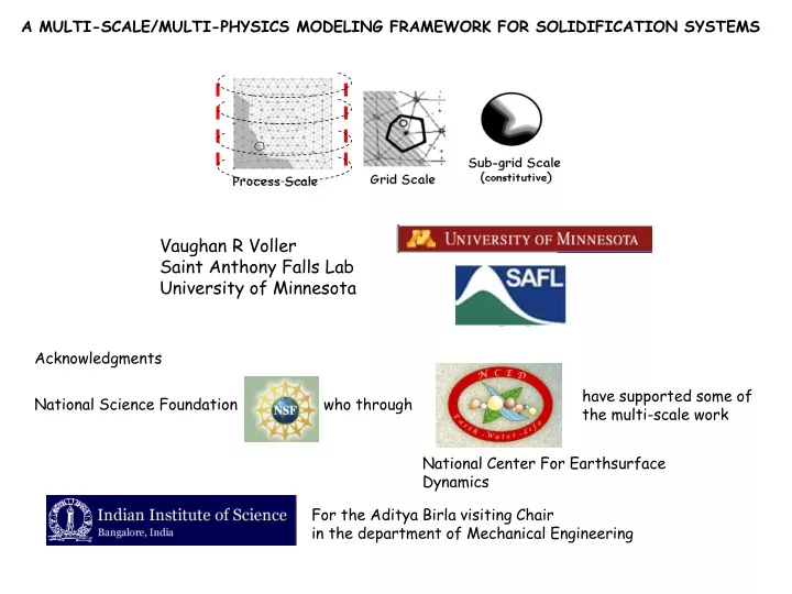
Acknowledgments. have supported some of the multi-scale work. National Science Foundation who through. National Center For Earthsurface Dynamics. For the Aditya Birla visiting Chair in the department of Mechanical Engineering.

E N D
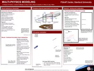
Acknowledgments have supported some of the multi-scale work National Science Foundation who through National Center For Earthsurface Dynamics For the Aditya Birla visiting Chair in the department of Mechanical Engineering A MULTI-SCALE/MULTI-PHYSICS MODELING FRAMEWORK FOR SOLIDIFICATION SYSTEMS Vaughan R Voller Saint Anthony Falls Lab University of Minnesota
KEY AREA OF INTEREST IN CFD Multi-physics –Multi-Scale 1. Process Optimization By blending models, plant/ field and experiment Experiment 2. Dovetailing Modeling and High Resolution Distributed Measurement Techniques Plant/field Data CFD- Model Flow + t e.g. optimization of wheel casting Cleary et al, Fluent LIDAR (1mm) measurement Of bed topography 3
Multi-physics –Multi-Scale Framework defines the domain of the problem Solidification Process (The Engineering) occur at the global scale of a product (~meters) Solidification Phenomena (The Science) occur at the local scale of the Solid Liquid Interface (~ microns) phenomena at scales below the grid resolution are incorporated into the analysis via the use of volume averaging and the development of constitutive relationships. Three Scales where nodal values of process variables are defined and stored To make progress in the “science” and “engineering” we need to bridge between these scales
Example: Macro-Segregation Scheil vs lever Distribution Of solute at scale of process
A microstructure model Growth of Equiaxed Crystal In under-cooled melt Sub-grid models Account for Crystal anisotropy and “smoothing” of interface jumps Phase change temperature depends on interface curvature, speed and concentration
Four fold symmetry If f= 0 or f = 1 If 0 < f < 1 curvature Capillary length 10-9 m in Al alloys Local direction In Detail Sub grid constitutive ENTHALPY Easy and Direct
At end of time step if solidification Completes in cell i Force solidification in ALL fully liquid neighboring cells. Some Results Physical domain ~ 2-10 microns Typical grid Size 200x200 ¼ geometry seed Initially insulated cavity contains liquid metal with bulk undercooling T0 < 0. Solidification induced by placing solid seed at center.
Dendrite shape with 3 grid sizes shows reasonable independence 3.25do (black) 4do (blue) 2.5do (red) e = 0.05, T0 = -0.65 Dimensionless time t = 6000 a = 0.25, b = 0.75
Tip Velocity Approaches Theoretical Limit at t =37,000, T0 = -0.55, e = 0.05, D= 2.5do ( ¼ box size 800x800)
Level Set Kim, Goldenfeld and Dantzig e = 0.05, T0 = -0.55, Dx = d0 Dimensionless time t = 37,600 Looks Right!! Verification 1 Enthalpy Calculation e = 0.05, T0 = -0.65, Dx = 3.333d0 Dimensionless time t = 0 (1000) 6000 Red my calculation for these parameters With grid size
Low Grid Anisotropy The Solid color is solved with a 45 deg twist on the anisotropy and then twisted back —the white line is with the normal anisotropy e = 0.05, T0 = -0.65 Dimensionless time t = 6000 Note: Different “smear” parameters are used in 00 and 450 case Tip position with time Not perfect: In 450 case the tip velocity at time 6000 (slope of line) is below the theoretical limit.
FAST-CPU This On This In 60 seconds ! time t = 6000 e = 0.05, T0 = -0.65 a = 0.25, b = 0.75, Dx =4d0
A Problem with Noise Grains in A Flow Field Thses calculations were performed by Andrew Kao, University of Greenwich, London Under supervision of Prof Koulis Pericleous and Dr. Georgi Djambazov. Playing Around Multiple Grains-multiple orientations
Have Presented Two examples of multi-scale multi-physics framework Can we Eliminate The middle Man An model Across Scales in One model? “Direct Microscale modeling” Model 1 Do we really want to do it? Model 2 100 10-9 Together they cover a vast range of scales
Update of Voller and Porte-Agel JCP 2003 3 Largest grid sizes (nodes/elements) reported in 11 MCWASP proceedings Dating back to 1980 and ending in 2006
Have Presented Two examples of multi-scale multi-physics framework In The mean time the Framework of Process-Grid-Sub-grid Is an adequate bridge Can produce insightful results And in some ways may provide more insight in to the process as opposed to a direct simulation!