Download
1 / 32
340 likes | 472 Views
Sect. 1.5: Probability Distribution for Large N. We’ve found that, for the one-dimensional Random Walk Problem , the probability distribution is the Binomial Distribution : W N (n 1 ) = [N!/(n 1 !n 2 !)]p n1 q n2 Here, q = 1 – p, n 2 = N - n 1

E N D
We’ve found that, for the one-dimensionalRandom Walk Problem, the probability distribution is theBinomial Distribution: WN(n1) = [N!/(n1!n2!)]pn1qn2 • Here, q = 1 – p, n2 = N - n1 The Relative Width:(Δ*n1)/<n1> = (q½)(pN)½ as N increases, the mean value increases N, & the relative width decreases (N)-½ N = 20, p = q = ½
Now, imagine Ngetting larger & larger. Based on what we just said, the relative width of WN(n1) gets smaller & smaller & the mean value <n1> gets larger & larger. • If N is VERY, VERY large, can treat W(n1) as a continuous function of a continuous variable n1. For N large, it’s convenient to look at the natural log ln[W(n1)] of W(n1), rather than the function itself. • Now, do a Taylor’s series expansion of ln[W(n1)] about value of n1 where W(n1) has a maximum. Detailed math (in the text) shows that this value of n1 is it’s average value <n1> = Np. It also shows that the width is equal to the value of the width <(Δn1)2> = Npq. • For ln[W(n1)], use Stirling’s Approximation(Appendix A-6) for logs of large factorials. Stirling’s Approximation If n is a large integer, the natural log of it’s factorial is approximately: ln[n!] ≈ n[ln(n) – 1]
In this large N, large n1 limit, the Binomial Distribution W(n1) becomes (shown in the text): W(n1) = Ŵexp[-(n1 - <n1>)2/(2<(Δn1)2>)] Here, Ŵ = [2π <(Δn1)2>]-½ • This is called the Gaussian Distribution or the Normal Distribution. We’ve found that <n1> = Np, <(Δn1)2> = Npq. • The reasoning which led to this for large N & continuous n1 limit started with theBinomial Distribution. However,this is a very general result. If one starts with ANYdiscrete probability distribution & takes the limit of LARGE N, one will obtain a Gaussian or Normal Distribution. This is called The Central Limit TheoremorThe Law of Large Numbers.
Sect. 1.6: Gaussian Probability Distributions • In the limit of a large number of steps in the random walk, N (>>1), the Binomial Distribution becomes a Gaussian Distribution: W(n1) = [2π<(Δn1)2>]-½exp[-(n1 - <n1>)2/(2<(Δn1)2>)] <n1> = Np, <(Δn1)2> = Npq • Recall that n1 = ½(N + m),where the displacement x = mℓ & that <m> = N(p – q). We can use this to convert to the probability distribution for displacement m, in the large N limit (after algebra): P(m) = [2π<(Δm)2>]-½exp[-(m- <m>)2/(2<(Δm)2>)] <m> = N(p – q), <(Δm)2> = 4Npq
P(m) = [2πNpq]-½exp[-(m – N{p – q})2/(8Npq)] We can express this in terms of x = mℓ.As N >> 1, xcan be treated as continuous. In this case, |P(m+2) – P(m)| << P(m) & discrete values of P(m) get closer & closer together. Now, lets ask: What is the probability that, after N steps, the particle is in the range x to x + dx? The probability distribution for this ≡ P(x). Then, we have: P(x)dx = (½)P(m)(dx/ℓ) The range dx contains (½)(dx/ℓ) possible values of m, since the smallest possible dxis dx = 2ℓ.
After some math, we obtain the standardGaussian Distributionform: P(x)dx = (2π)-½σ-1exp[-(x – μ)2/2σ2] Here: μ ≡ N(p – q)ℓ ≡ mean value of x σ ≡ 2ℓ(Npq)-½ ≡width of the distribution NOTE:The generality of the arguments we’ve used is such that aGaussian distribution occurs in the limit of large numbers for any discrete distribution
P(x)dx = (2π)-½σ-1exp[-(x – μ)2/2σ2] μ ≡ N(p – q)ℓσ ≡ 2ℓ(Npq)-½ • Note:To deal with Gaussian distributions, you need to get used to doing integrals with them! Many of these are tabulated!! • Is P(x)properly normalized? That is, does P(x)dx = 1? (limits - < x < ) P(x)dx = (2π)-½σ-1exp[-(x – μ)2/2σ2]dx = (2π)-½σ-1exp[-y2/2σ2]dy (y = x – μ) = (2π)-½σ-1 [(2π)½σ] (from a table) P(x)dx = 1
P(x)dx = (2π)-½σ-1exp[-(x – μ)2/2σ2] μ ≡ N(p – q)ℓσ ≡ 2ℓ(Npq)-½ • Compute the mean value of x (<x>): <x> = xP(x)dx = (limits - < x < ) xP(x)dx = (2π)-½σ-1xexp[-(x – μ)2/2σ2]dx = (2π)-½σ-(y + μ)exp[-y2/2σ2]dy(y = x – μ) = (2π)-½σ-1yexp[-y2/2σ2]dy + μ exp[-y2/2σ2]dy yexp[-y2/2σ2]dy = 0(odd function times even function) exp[-y2/2σ2]dy = [(2π)½σ] (from a table) <x> = μ ≡ N(p – q)ℓ
P(x)dx = (2π)-½σ-1exp[-(x – μ)2/2σ2] μ ≡ N(p – q)ℓσ ≡ 2ℓ(Npq)-½ • Compute the dispersion in x (<(Δx)2>) <(Δx)2> = <(x – μ)2> = (x – μ)2P(x)dx = (limits - < x < ) xP(x)dx = (2π)-½σ-1xexp[-(x – μ)2/2σ2]dx = (2π)-½σ-1y2exp[-y2/2σ2]dy(y = x – μ) = (2π)-½σ-1(½)(π)½σ(2σ2)1.5(from table) <(Δx)2> = σ2 = 4Npqℓ2
Comparison of Binomial & Gaussian Distributions Dots: Binomial Curve: Gaussian The same mean & the same width
Sect. 1.7: Probability Distributions Involving Several Variables
Consider a statistical description of a situation with more than one variable:For example, 2 variables, u, v The possible values of u are: u1,u2,u3,…uM The possible values ofv are: v1,v2,v3,…vM Let P(ui,vj) ≡ Probability thatu = ui, &v = vjsimultaneously • We must have: ∑i = 1 M ∑j = 1 NP(ui,vj) = 1 • Pu(ui) ≡ Probability thatu = ui independent of value v = vjPu(ui) ≡ ∑j = 1 NP(ui,vj) • Pv(vj) ≡ Probability that v = vjindependent of value u = uiPv(vj) ≡ ∑i = 1 MP(ui,vj) • Of course, ∑i = 1 M Pu(ui) = 1 &∑j = 1 NPv(vj) = 1
In the special casethat u, v are Statistically Independent or Uncorrelated: Then & only then: P(ui,vj) ≡ Pu(ui)Pv(vj) General Discussion of Mean Values: • If F(u,v) = any function ofu,v, it’s mean value is given by: <F(u,v)> ≡ ∑i = 1 M ∑j = 1 NP(ui,vj)F(ui,vj) • If F(u,v) & G(u,v) are any 2 functions ofu,v, can easily show: <F(u,v) + G(u,v)>= <F(u,v)> + <G(u,v)> • If f(u) is any function of u& g(v)> is any function ofv, we can easily show: <f(u)g(v)>≠ <f(u)><g(v)> The only case when the inequality becomes an equality is if u& v are statistically independent.
Sect. 1.8: Comments on Continuous Probability Distributions • Everything we’ve discussed for discrete distributions generalizes in obvious ways. • u ≡ a continuous random variable in the range: a1≤ u ≤ a2 • The probability of finding u in the range u to u + du≡ P(u) ≡ P(u)du P(u)≡Probability Densityof the distribution function • Normalization: P(u)du= 1 (limitsa1≤ u ≤ a2) • Mean values: <F(u)> ≡F(u)P(u)du.
Consider two continuous random variables: u ≡ continuous random variable in range: a1≤ u ≤ a2 v ≡ continuous random variable in range: b1≤ v ≤ b2 • The probability of finding u in the range u to u + duAND v in the range v to v + dvis P(u,v) ≡ P(u,v)dudv P(u,v) ≡Probability Densityof the distribution function • Normalization: P(u,v)dudv= 1(limitsa1≤ u ≤ a2, b1≤ v ≤ b2) • Mean values: <G(u,v)> ≡G(u,v)P(u,v)dudv
Functions of Random Variables An important, often occurring problem: Consider a random variable u. Suppose φ(u)≡ any continuous function of u. Question: If P(u)du ≡Probability of finding u in the range u to u + du, what is the probability W(φ)dφ of finding φin the range φto φ + dφ? • Answer by using essentially the “Chain Rule” of differentiation, but take the absolute value to make sure thatW ≥ 0: W(φ)dφ ≡ P(u)|du/dφ|dφ Caution!!φ(u)may not be a single valued function of u!
Equally Likely The probability of finding θbetween θ & θ + dθis: P(θ)dθ ≡ (dθ/2π) Question: What is the probability W(Bx)dBxthat the x component of B lies between Bx & Bx + dBx? Clearly, we must have –B ≤ Bx ≤ B. Also, each value of dBx corresponds to 2 possible values of dθ. Also, dBx = |Bsinθ|dθ • Example: A 2-dimensional vector B of constant magnitude|B| is EQUALLY LIKELY to point in any direction θ in the x-y plane. Figures
So, we have: W(Bx)dBx = 2P(θ)|dθ/dBx|dBx = (π)-1dBx/|Bsinθ| Note also that: |sinθ| = [1 – cos2θ]½= [1 – (Bx)2/B2]½so finally, W(Bx)dBx = (π)-1dBx[1 – (Bx)2/B2]-½, –B ≤ Bx ≤ B = 0, otherwise W not only has a maximum at Bx = B,it diverges there! It has a minimum at Bx = 0. So, it looks like Wdiverges at Bx = B, but it can be shown that it’s integral is finite. So, thatW(Bx)is a proper probability: W(Bx)dBx= 1 (limits:–B ≤ Bx ≤ B)
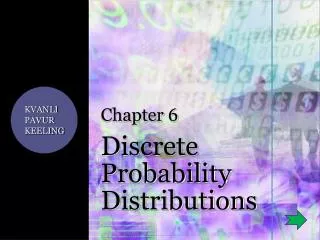
The Poisson Probability Distribution Simeon Denis Poisson • "Researches on the probability of criminal and civil verdicts" 1837 • Looked at the form of the binomial distribution when the number of trials is large. • He derived the cumulative Poisson distribution as the limiting case of the binomial when the chance of success tends to zero.
The Poisson Probability Distribution Simeon Denis Poisson • "Researches on the probability of criminal and civil verdicts" 1837 • Looked at the form of the binomial distribution when the number of trials is large. • He derived the cumulative Poisson distribution as the limiting case of the binomial whenthe chance of success tends to zero. Simeon Denis “Fish”!
Another Useful Probability Distribution:The Poisson Distribution • Poisson Distribution: Approximation to binomial distribution for the special casewhen the average number of successes is very much smaller than the possible numberi.e.µ << n because p << 1. • It is important for the study of such phenomena as radioactive decay. This distribution is NOTnecessarily symmetric! Data are usually bounded on one side and not the other. An advantage of this distribution is that σ2 = μ µ = 10.0 σ = 3.16 µ = 1.67 σ = 1.29
The Poisson Distribution models counts:If events happen at a constant rate over time, the Poisson distribution gives the probability of X number of events occurring in a time T. • This distribution tells us the probability of all possible numbers of counts, from 0 to infinity. • If X= # of counts per second, then the Poisson probability that X = k(a particular count) is: • Here, λ ≡ the average number of counts per second.
Mean and Variance for the Poisson Distribution • It’s easy to show that: The Mean The Variance & Standard Deviation For a Poisson Distribution, the variance and mean are the same!
More on the Poisson Distribution Terminology: A “Poisson Process” • The Poisson parameter can be given as the mean number of events that occur in a defined time period OR, equivalently, can be given as a rate, such as = 2 events per month. must often be multiplied by a time t in a physical process (called a “Poisson Process”) μ = t σ = t
Example 1.If calls to your cell phone are a Poisson process with a constant rate = 2 calls per hour, what is the probability that, if you forget to turn your phone off in a 1.5 hour movie, your phone rings during that time? Answer:If X = # calls in 1.5 hours, we want P(X ≥ 1) = 1 – P(X = 0) P(X ≥ 1) = 1 – .05 = 95% chance 2.How many phone calls do you expect to get during the movie? <X> = t = 2(1.5) = 3 Editorial comment:People at the movie will not be very happy with you!!
Conditions required for the Poisson Distribution to hold: The rate is a constant, independent of time. Two eventsnever occurat exactly the same time. Each event is independent --- the occurrence of one event does not make the next event more or less likely to happen. 31
Example • A production line produces 600 parts per hour with an average of 5 defective parts an hour. If you test every part that comes off the line in 15 minutes, what is the probability of finding no defective parts (and incorrectly concluding that your process is perfect)? = (5 defects/hour)*(0.25 hour) = 1.25 p(x) = (xe-)/(x!) x = given number of defects P(x = 0) = (1.25)0e-1.25)/(0!) = e-1.25 = 0.287 = 28.7%