Download
1 / 80
820 likes | 1.05k Views
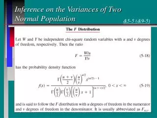
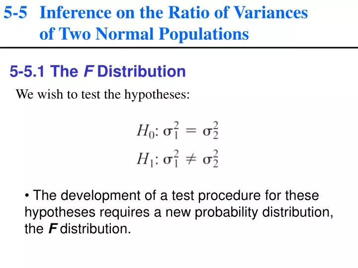
5-5 Inference on the Ratio of Variances of Two Normal Populations. 5-5.1 The F Distribution. We wish to test the hypotheses:. The development of a test procedure for these hypotheses requires a new probability distribution, the F distribution.

E N D
5-5 Inference on the Ratio of Variances of Two Normal Populations 5-5.1 The F Distribution We wish to test the hypotheses: • The development of a test procedure for these hypotheses requires a new probability distribution, the Fdistribution.
5-5 Inference on the Ratio of Variances of Two Normal Populations 5-5.1 The F Distribution
5-5 Inference on the Ratio of Variances of Two Normal Populations 5-5.1 The F Distribution
5-5 Inference on the Ratio of Variances of Two Normal Populations The Test Procedure
5-5 Inference on the Ratio of Variances of Two Normal Populations The Test Procedure
5-5 Inference on the Ratio of Variances of Two Normal Populations The Test Procedure
5-5 Inference on the Ratio of Variances of Two Normal Populations Example 5-10 OPTIONS NOOVP NODATE NONUMBER LS=80; DATA; n1=15; n2=15; alpha=0.05; df1=n1-1; df2=n2-1; s1=1.96; s2=2.13; f0=(s1**2)/(s2**2); pvalue=2*probf(f0, df1, df2); f=finv(pvalue/2, df1, df2); f1=1-probf(f0, df2, df1); f2=1/f1; CL=f0*f1; CU=f0*f2; PROCPRINT; var f0 df1 df2 pvalue f f1 f2 CL CU; RUN; QUIT; OBS f0 df1 df2 p-value f f1 f2 CL CU 1 0.84675 14 14 0.75995 0.84675 0.62002 1.61284 0.52500 1.36566
5-5 Inference on the Ratio of Variances of Two Normal Populations 5-5.2 Confidence Interval on the Ratio of Two Variances
5-5 Inference on the Ratio of Variances of Two Normal Populations
5-5 Inference on the Ratio of Variances of Two Normal Populations
5-6 Inference on Two Population Proportions 5-6.1 Hypothesis Testing on the Equality of Two Binomial Proportions
5-6 Inference on Two Population Proportions 5-6.1 Hypothesis Testing on the Equality of Two Binomial Proportions
5-6 Inference on Two Population Proportions
5-6 Inference on Two Population Proportions
5-6 Inference on Two Population Proportions
5-6 Inference on Two Population Proportions OPTIONS NOOVP NODATE NONUMBER LS=80; DATA EX512; N1=300; N2=300; ALPHA=0.05; DFT1=253; DFT2=196; P1HAT=DFT1/N1; P2HAT=DFT2/N2; DIFFP=P1HAT-P2HAT; PHAT=(DFT1+DFT2)/(N1+N2); Z0=DIFFP/SQRT(PHAT*(1-pHAT)*(1/N1+1/N2)); PVALUE=2*(1-PROBNORM(Z0)); ZVALUE=ABS(PROBIT(ALPHA/2)); LIMIT=ZVALUE*SQRT((P1HAT*(1-P1HAT)/N1) + (P2HAT*(1-p2HAT)/N2)); UL=DIFFP+LIMIT; LL=DIFFP-LIMIT; PROCPRINT; var P1HAT P2HAT DIFFP PHAT Z0 ZVALUE PVALUE LL UL; RUN; QUIT; OBS P1HAT P2HAT DIFFP PHAT Z0 ZVALUE PVALUE LL UL 1 0.84333 0.65333 0.19 0.74833 5.36215 1.95996 8.2238E-8 0.12224 0.25776
5-6 Inference on Two Population Proportions 5-6.2 Type II Error and Choice of Sample Size
5-6 Inference on Two Population Proportions 5-6.2 Type II Error and Choice of Sample Size
5-6 Inference on Two Population Proportions 5-6.2 Type II Error and Choice of Sample Size
5-8 What If We Have More Than Two Samples? 5-8.1 Completely Randomized Experiment and Analysis of Variance (Replicates) Treatments
5-8 What If We Have More Than Two Samples? 5-8.1 Completely Randomized Experiment and Analysis of Variance • The levels of the factor are sometimes called treatments. • Each treatment has six observations or replicates. • The runs are run in random order.
5-8 What If We Have More Than Two Samples? 5-8.1 Completely Randomized Experiment and Analysis of Variance
5-8 What If We Have More Than Two Samples? 5-8.1 Completely Randomized Experiment and Analysis of Variance = + =0
5-8 What If We Have More Than Two Samples? 5-8.1 Completely Randomized Experiment and Analysis of Variance
5-8 What If We Have More Than Two Samples? 5-8.1 Completely Randomized Experiment and Analysis of Variance
5-8 What If We Have More Than Two Samples?
5-8 What If We Have More Than Two Samples? 5-8.1 Completely Randomized Experiment and Analysis of Variance
5-8 What If We Have More Than Two Samples? 5-8.1 Completely Randomized Experiment and Analysis of Variance
5-8 What If We Have More Than Two Samples?
5-8 What If We Have More Than Two Samples? 5-8.1 Completely Randomized Experiment and Analysis of Variance
5-8 What If We Have More Than Two Samples? Which means differ?
5-8 What If We Have More Than Two Samples? Multiple Comparisons If we wish to make all pairwise comparisons we need to worry about the probability of a type I error on each test and also the probability of making at least one type I error on all the tests. This latter error is referred to as the experiment-wise error rate or the overall error rate. A number of procedures are available to protect the overall error rate. They all compare the differences to a cut-off value. The cut-off values all have the form
5-8 What If We Have More Than Two Samples? • Steps in Multiple Comparisons • Calculate . • Determine cut-off. Any difference in 1) larger than the cut-off have corresponding means that are significantly different from one another. • Fisher’s Least Significant Difference (LSD). This does not protect the overall error rate. The overall error rate will be approximately , where c is the number of comparisons being made. • If all then
5-8 What If We Have More Than Two Samples? • Steps in Multiple Comparisons • Tukey’s Highest Significance Difference (HSD). This controls overall error rate. The overall error rate will be a. • If all then • An alternative in unbalanced designs is • With Tukey’s you need both the degrees of freedom (n – r) and also the number of means being compared (r).
5-8 What If We Have More Than Two Samples? • Steps in Multiple Comparisons • Student’s, Neuman’s, Keuls (SNK). • This overall error rate is between that of Fisher’s and Tukey’s. • d is the number of means apart the two means being compared are in the ordered list of means (d between 2 and r). Notice, more than one cut-off is needed for the SNK. The SNK is done sequentially, starting with the means the farthest apart. Once a pair of means is found to be not significantly different, all pairs closer together are deemed not significantly different.
5-8 What If We Have More Than Two Samples?
5-8 What If We Have More Than Two Samples? Residual Analysis and Model Checking
5-8 What If We Have More Than Two Samples? Residual Analysis and Model Checking
5-8 What If We Have More Than Two Samples? Residual Analysis and Model Checking
5-8 What If We Have More Than Two Samples? Residual Analysis and Model Checking
5-8 What If We Have More Than Two Samples? OPTIONS NOOVP NODATE NONUMBER LS=80; proc format; value hc 1=' 5%' 2='10%' 3='15%' 4='20%'; DATA ex514; INPUT hc strength @@; format hchc.; CARDS; 1 7 2 12 3 14 4 19 1 8 2 17 3 18 4 25 1 15 2 13 3 19 4 22 1 11 2 18 3 17 4 23 1 9 2 19 3 16 4 18 1 10 2 15 3 18 4 20 procanova data=ex514; class hc; model strength= hc; means hc/lsdsnktukey; TITLE 'procanova balanced 1-way anova'; proc sort; by hc; proc boxplot; plot strength*hc; procglm data=ex514; class hc; model strength= hc; means hc/lsdsnktukey; output out=new p=phat r=resid; TITLE 'procglm 1-way anova'; procplot data=new; plot resid*(phathc); Title 'Residual plot'; RUN; QUIT;
5-8 What If We Have More Than Two Samples? procanova balanced 1-way anova The ANOVA Procedure Class Level Information Class Levels Values hc 4 5% 10% 15% 20% Number of Observations Read 24 Number of Observations Used 24 procanova balanced 1-way anova The ANOVA Procedure Dependent Variable: strength Sum of Source DF Squares Mean Square F Value Pr > F Model 3 382.7916667 127.5972222 19.61 <.0001 Error 20 130.1666667 6.5083333 Corrected Total 23 512.9583333 R-Square CoeffVar Root MSE strength Mean 0.746243 15.98628 2.551144 15.95833 Source DF Anova SS Mean Square F Value Pr > F hc 3 382.7916667 127.5972222 19.61 <.0001
5-8 What If We Have More Than Two Samples? procanova balanced 1-way anova The ANOVA Procedure t Tests (LSD) for strength NOTE: This test controls the Type I comparisonwise error rate, not the experimentwise error rate. Alpha 0.05 Error Degrees of Freedom 20 Error Mean Square 6.508333 Critical Value of t 2.08596 Least Significant Difference 3.0724 Means with the same letter are not significantly different. t Grouping Mean N hc A 21.167 6 20% B 17.000 6 15% B 15.667 6 10% C 10.000 6 5%
5-8 What If We Have More Than Two Samples? procanova balanced 1-way anova The ANOVA Procedure Student-Newman-Keuls Test for strength NOTE: This test controls the Type I experimentwise error rate under the complete null hypothesis but not under partial null hypotheses. Alpha 0.05 Error Degrees of Freedom 20 Error Mean Square 6.508333 Number of Means 2 3 4 Critical Range 3.0724227 3.726419 4.1225627 Means with the same letter are not significantly different. SNK Grouping Mean N hc A 21.167 6 20% B 17.000 6 15% B 15.667 6 10% C 10.000 6 5%
5-8 What If We Have More Than Two Samples? procanova balanced 1-way anova The ANOVA Procedure Tukey'sStudentized Range (HSD) Test for strength NOTE: This test controls the Type I experimentwise error rate, but it generally has a higher Type II error rate than REGWQ. Alpha 0.05 Error Degrees of Freedom 20 Error Mean Square 6.508333 Critical Value of Studentized Range 3.95829 Minimum Significant Difference 4.1226 Means with the same letter are not significantly different. Tukey Grouping Mean N hc A 21.167 6 20% B 17.000 6 15% B 15.667 6 10% C 10.000 6 5%
5-8 What If We Have More Than Two Samples?
5-8 What If We Have More Than Two Samples? procglm 1-way anova The GLM Procedure Dependent Variable: strength Sum of Source DF Squares Mean Square F Value Pr > F Model 3 382.7916667 127.5972222 19.61 <.0001 Error 20 130.1666667 6.5083333 Corrected Total 23 512.9583333 R-Square CoeffVar Root MSE strength Mean 0.746243 15.98628 2.551144 15.95833 Source DF Type I SS Mean Square F Value Pr > F hc 3 382.7916667 127.5972222 19.61 <.0001 Source DF Type III SS Mean Square F Value Pr > F hc 3 382.7916667 127.5972222 19.61 <.0001
5-8 What If We Have More Than Two Samples? Residual plot resid*phat도표. 범례: A = 1 관측치, B = 2 관측치, 등. resid | | 5.000 + A 4.500 + 4.000 + 3.500 + A 3.000 + A 2.500 + A 2.000 + A 1.500 + A A 1.000 + A B 0.500 + A 0.000 + A A -0.500 + A -1.000 + A A -1.500 + A -2.000 + A -2.500 + A A -3.000 + A A -3.500 + A -3.667 + A | ---+----------+----------+----------+----------+----------+----------+-- 10 12 14 16 18 20 22 phat Residual plot resid*hc도표. 범례: A = 1 관측치, B = 2 관측치, 등. resid | | 5.000 + A 4.500 + 4.000 + A 3.500 + A 3.000 + 2.500 + A 2.000 + A 1.500 + A A 1.000 + A B 0.500 + A 0.000 + A A -0.500 + A -1.000 + A A -1.500 + A -2.000 + A A -2.500 + A -3.000 + A A -3.500 + A -3.667 + A | ---+-----------------+-----------------+-----------------+-- 5% 10% 15% 20% hc
5-8 What If We Have More Than Two Samples? Kruskal-Wallis Nonparametric Test H0: All k populations have the same distribution H1: Not all populations have the same distribution. Test Statistic: Here the Ri are the sum of the ranks for each population. The ranks are found by ranking the data in all populations combined. The n is the total sample size and ni is the sample size of the sample from the ith population. Rejection Region: Paired comparison of population i to j:
5-8 What If We Have More Than Two Samples? Example An article in Fortune compared rent in five American cities: New York, Chicago, Detroit, Tampa, and Orlando. The following data are small random samples of rants (in dollars) in the five cities. The New York data are Manhattan only. Conduct the Kruskal-Wallis test to determine whether evidence exists that there are significant differences in the rents in these cities. If differences exit, where are they? OPTIONS NOOVP NODATE NONUMBER LS=80; procformat; value city 1=' New York' 2='Chicago' 3='Detroit' 4='Tampa' 5='Orlando'; DATA rent; INPUT city rent @@; format city city.; CARDS; 1 900 1 1200 1 850 1 1320 1 1400 1 1150 1 975 2 625 2 640 2 775 2 1000 2 690 2 550 2 840 2 750 3 415 3 400 3 420 3 560 3 780 3 620 3 800 3 390 4 410 4 310 4 320 4 280 4 500 4 385 4 440 5 340 5 425 5 275 5 210 5 575 5 360 procnpar1way data=rent wilcoxon; class city; var rent; TITLE 'Kruskal-Wallis Test'; RUN; QUIT; Kruskal-Wallis Test The NPAR1WAY Procedure Wilcoxon Scores (Rank Sums) for Variable rent Classified by Variable city Sum of Expected StdDev Mean city N Scores Under H0 Under H0 Score -------------------------------------------------------------------------------- New York 7 228.0 129.50 25.018327 32.571429 Chicago 8 192.0 148.00 26.280538 24.000000 Detroit 8 135.0 148.00 26.280538 16.875000 Tampa 7 62.0 129.50 25.018327 8.857143 Orlando 6 49.0 111.00 23.558438 8.166667 Kruskal-Wallis Test Chi-Square 26.4930 DF 4 Pr > Chi-Square <.0001