Download
1 / 46
460 likes | 479 Views
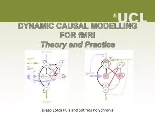
Methods for Dummies 2010. Dynamic Causal Modelling for fMRI. Justin Grace Marie-Hélène Boudrias. DCM Motivation. Dynamic Causal Modelling (DCM) was born out of a simple problem:

E N D
Methods for Dummies 2010 Dynamic Causal Modelling for fMRI Justin Grace Marie-Hélène Boudrias
DCM Motivation Dynamic Causal Modelling (DCM) was born out of a simple problem: • Cognitive neuroscientists want to talk about activation at the level of neuronal systems in order to hypothesize about cognitive processes • Imaging techniques do not generate data at this level, but give output relating to non-linear correlates, such as haemodynamics (BOLD signal) in the case of fMRI • Moreover, it would be useful to be able to talk about causality in neuronal populations, since we know that signals propagate in a wave-like manner from some input through a system • DCM attempts to tackle these problems
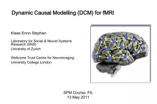
DCM History • Introduced in 2002 for fMRI data (Friston, 2002) • DCM is a generic approach for inferring hidden (unobserved) neuronal states from measured brain activity. • The mathematical basis and implementation of DCM for fMRI have since been refined and extended repeatedly. • DCMs have also been implemented for a range of measurement techniques other than fMRI, including EEG, MEG (to be presented next week), and LFPs obtained from invasive recordings in humans or animals.
Recap on Connectivity • Structural connectivity – the physical structure of the brain • Functional connectivity – the likelihood that 2 neuronal populations share associated activity • Effective connectivity – a union between structural and functional connectivity. • => DCM • Structural, functional, and effective connectivity matrices. • Binary or Non-binary – reflecting proximity between elements (presence or magnitude respectively) • Symmetrical or Non-symmetrical – reflecting direction independence, or directional effects respectively
Overview • Dynamic causal models (DCMs) • Basic idea • Neural level • haemodynamic level • Priors & Parameter estimation • Rules of good practice of DCM with fMRI data
Basic Idea • DCM allows us to model interactions among neuronal populations at a cortical level using approximations of neural activity. Today, since we are discussing DCM using fMRI, our source data reflects the haemodynamic time series. • Using these models we can begin to make inferences about the coupling among brain areas, & how that coupling can be manipulated by changes to the experimental context. • This approach requires several components that build on prior knowledge about that brain & neural systems established by previous research…
y y y y y The aim of DCM Functional integration and the modulation of specific pathways Intrinsic connections Based on prior data & concrete hypotheses A Matrix Contextual inputs Stimulus-free - u(t) {e.g. cognitive set/time} B Matrix BA39 Perturbing inputs Stimuli-bound u1(t) {e.g. visual words} C Matrix STG V4 V1 BA37
Basics of Dynamic Causal Modelling • DCM allows us to look at how areas within a network interact: • Investigate functional integration & modulation of specific cortical pathways • Temporal dependency of activity within and between areas (causality)
Temporal dependence and causal relations Seed voxel approach, PPI etc. Dynamic Causal Models T0 T1 T2 …. T0 T1 T2 …. timeseries (neuronal activity)
What is a system? Input u(t) System = a set of elements which interact in a spatially and temporally specific fashion connectivity parameters systemstate z(t) • State changes of a system are dependent on: • the current state • external inputs • its connectivity • time constants & delays
Linear Dynamic Model X1= A11X1 + A21X2 + C11U1 X2= A22X2 + A12X1 + C22U2 The Linear Approximation fL(x,u)=Ax + Cu Intrinsic Connectivity Extrinsic (input) Connectivity
Bi-Linear Dynamic Model (DCM) X1= A11X1 + (A21+ B212U1(t))X+ C11U1 X2= A22X2 + A12X1 + C22U2 The Bilinear Approximation fB(x,u)=(A+jUjBj)x + Cu Intrinsic Connectivity Extrinsic (input) Connectivity INDUCED CONNECTIVITY
Neurodynamics: 2 nodes with input u1 u2 u1 z1 z1 z2 z2 activity in z2 is coupled to z1 via coefficient a21
Neurodynamics: positive modulation u1 u1 u2 u2 z1 z1 z2 z2 index, not squared modulatory input u2 activity through the coupling a21
Neurodynamics: reciprocal connections u1 u1 u2 u2 z1 z1 z2 z2 reciprocal connection disclosed by u2
Neuronal level summary This completes the neuronal model – hopefully you now have some understanding as to how the neuronal model generates output relating to neuronal activity. we have explained how any 2 elements of interest interact with each other and the stimulus input; How elements can be combined to talk about a neuronal system state; And how we can identify change in this system over time; In order to discuss intrinsic and induced connectivity with respect to extrinsic stimulus effects.
Basics of Dynamic Causal Modelling • DCM allows us to look at how areas within a network interact: • Investigate functional integration & modulation of specific cortical pathways • Temporal dependency of activity within and between areas (causality) • Separate neuronal activity from observed BOLD responses
x λ y Basics of DCM: Neuronal and BOLD level • Cognitive system is modelled at its underlying neuronal level (not directly accessible for fMRI). • The modelled neuronal dynamics (x) are transformed into area-specific BOLD signals (y) by a haemodynamicmodel (λ). The aim of DCM is to estimate parameters at the neuronal level such that the modelled and measured BOLD signals are maximally* similar.
t The haemodynamic model u stimulus functions • 6 haemodynamic parameters: neural state equation important for model fitting, but of no interest for statistical inference haemodynamic state equations • Computed separately for each area region-specific HRFs! Estimated BOLD response Friston et al. 2000, NeuroImage Stephan et al. 2007, NeuroImage
Haemodynamics: reciprocal connections u1 BOLD (without noise) u2 h1 z1 BOLD (without noise) h2 z2 blue: neuronal activity red: BOLD response h(u,θ) represents the BOLD response (balloon model) to input
Haemodynamics: reciprocal connections u1 BOLD with Noise added u2 y1 z1 BOLD with Noise added y2 z2 blue: neuronal activity red:BOLD response y represents simulated observation of BOLD response, i.e. includes noise
So we now have models of BOLD signal output based on our predicted neuronal model. Marie-Hélène will describe the process of setting these models with appropriate priors and using parameter estimation to identify the most appropriate model.
Overview • Dynamic causal models (DCMs) • Basic idea • Neural level • Hemodynamic level • Parameter estimation, priors & inference • Rules of good practice of DCM with fMRI data
Neuronal dynamics Haemodynamics State space Model Priors Posterior densities of parameters Bayesian Model inversion fMRI data Model comparison Dynamic Causal Modelling of fMRI DCM roadmap
stimulus function u Overview:parameter estimation neuronal state equation • Specify model (neuronal and haemodynamic level). • Bayesian parameter estimation to minimise difference between data and model. • Result:Gaussian a posteriori coupling parameter distributions, characterised by mean ηθ|y and covariance Cθ|y. hemodynamic state equations parameters ηθ|y modeled BOLD response
Measured vs Modelled BOLD signal • The aim of DCM is to estimate • neural parameters {A, B, C} • hemodynamic parameters • such that the modelled and measured BOLD signals are maximally similar.
Estimation: Bayesian framework • Models of • Combined haemodynamics and • neural parameter set • Constraints on • Haemodynamic parameters • Connections (coupling parameters) prior likelihood term posterior The posterior probability of the parameters given the data is an optimal combination of prior knowledge and new data, weighted by their relative precision. Bayesian estimation
Interpretation of parameters • The model parameters are distributions that have a mean ηθ|y and covariance Cθ|y . • Quantify the probability that a parameter (ηθ|y) is above a chosen threshold γ: ηθ|y • By default, γ is chosen as zero • ("does this coupling parameter exist?").
Bayesian Model Selection (BMS) • Model evidence involves integrating out the dependency of the model parameters: • BMS is an established procedure in statistics that rests on computing the model evidence • i.e., the probability of the data y, given some model m. • The model evidence, which can be considered the “holy grail” of model comparison, quantifies the properties of a good model. • It explains the data as accurately as possible and, at the same time, has minimal complexity.
Model comparison Given competing hypotheses on structure & functional mechanisms of a system, which model is the best? Which model represents thebest balance between model fit and model complexity? For which model m does p(y|m) become maximal?
Bayesian Model Selection (BMS) • In BMS, models are usually compared via their Bayes factor, • i.e., the ratio of their respective evidences: • The “Bayes factor” is a summary of the evidence in favour of one model as opposed to another. • i.e. Given candidate models m1and m2, a Bayes factor of 20 corresponds to a belief of 95% in the statement ‘m1 is better than m2’.
Overview • Dynamic causal models (DCMs) • Basic idea • Neural level • Hemodynamic level • Parameter estimation, priors & inference • Rules of good practice of DCM with fMRI data
Rules of good practice • DCM is dependent on experimental perturbations • Experimental conditions enter the model as inputs that either drive the local responses or change connections strengths. • If there is no evidence for an experimental effect (no activation detected by a GLM) → inclusion of this region in a DCM is not meaningful. • Use the same optimization strategies for design and data acquisition that apply to conventional GLM of brain activity: • preferably multi-factorial (e.g. 2 x 2) • one factor that varies the driving (sensory) input • one factor that varies the contextual input
Define the relevant model space • Define sets of models that are plausible, given prior knowledge about the system, this could be e.g.: • derived from principled considerations • informed by previous empirical studies using neuroimaging, electrophysiology, TMS, etc. in humans or animals. • Use anatomical information and computational models to refine your DCMs. • The definition of the relevant model space should be as transparent and systematic as possible, and it should be described clearly in any article.
Motivate model space carefully • Models are never true; by construction, they are meant to be helpful caricatures of complex phenomena, such that mechanisms underlying these phenomena can be tested. • The purpose of model selection is to determine which model, from a set of plausible alternatives, is most useful i.e., represents the best balance between accuracy and complexity. • The critical question in practice is how many plausible model alternatives exist? • For small systems (i.e., networks with a small number of nodes), it is possible to investigate all possible connectivity architectures. • With increasing number of regions and inputs, evaluating all possible models becomes practically impossible very rapidly.
What you can not do with BMS • Model evidence is defined with respect to one particular data set. This means that BMS cannot be applied to models that are fitted to different data. • Specifically, in DCM for fMRI, one cannot compare models with different numbers of regions, because changing the regions changes the data. • Maximum of 8 regions with SPM8.
Fig. 1. This schematic summarizes the typical sequence of analysis in DCM, depending on the question of interest. Abbreviations: FFX=fixed effects, RFX=random effects, BMS=Bayesian model selection, BPA=Bayesian parameter averaging, BMA=Bayesian model averaging, ANOVA=analysis of variance. 10 Simple Rules for DCM (2010). Stephan et al. NeuroImage 52.
BA39 Perturbing inputs C matrix STG V4 y y y y y V1 BA37
Fig. 1. This schematic summarizes the typical sequence of analysis in DCM, depending on the question of interest. Abbreviations: FFX=fixed effects, RFX=random effects, BMS=Bayesian model selection, BPA=Bayesian parameter averaging, BMA=Bayesian model averaging, ANOVA=analysis of variance. 10 Simple Rules for DCM (2010). Stephan et al. NeuroImage 52.
Contextual inputs B matrix BA39 Perturbing inputs C matrix STG V4 y y y y y V1 BA37
PMd PMd SMA PMv PMv SMA M1 M1 Practical steps of DCM Design matrix 1) Standard Analysis of fMRI Data 2) Statistical Parametric Maps - Extract times series from chosen areas 3) Construction of a Connectivity Model - Add a forward model of how neuronal activity causes the signals you observe (e.g. BOLD) (Neural and hemodynanics models) 4) Evaluation of the Connectivity Model - Estimation of the parameters in your model (effective connectivity), given your observed data 5) BMS, BMA or BPA SPMs
PMd PMd PMv SMA PMv SMA M1 M1 ηθ|y0 Left Right A Matrix = rate constant in 1/s or Hz - Coupling represents the connection strength describing how fast and strong a response occur in the target region. - If M1_LPMd_L is 0.36 s-1 this means that, per unit time, the increase in activity in PMd_L corresponds to 36% of the activity in M1_L. • B Matrix = Used to calculate the % of change of connection strength in the target region by the factor that varies the contextual input. C Matrix = Entrance of the driving (sensory) input in the network
So, DCM…. • enables one to infer hidden neuronal processes from fMRI data • tries to model the same phenomena as a GLM • explaining experimentally controlled variance in local responses • based on connectivity and its modulation • allows one to test mechanistic hypotheses about observed effects • is informed by anatomical and physiological principles. • uses a Bayesian framework to estimate model parameters • is a generic approach to modelling experimentally perturbed dynamic systems. • provides an observation model for neuroimaging data, e.g. fMRI, M/EEG
The first DCM paper: Dynamic Causal Modelling (2003). Friston et al.NeuroImage 19:1273-1302. • Physiological validation of DCM for fMRI: Identifying neural drivers with functional MRI: an electrophysiological validation (2008). David et al. PLoS Biol. 6 2683–2697 • Hemodynamic model: Comparing hemodynamic models with DCM (2007). Stephan et al. NeuroImage 38:387-401 • Nonlinear DCMs:Nonlinear Dynamic Causal Models for FMRI (2008). Stephan et al. NeuroImage 42:649-662 • Two-state model: Dynamic causal modelling for fMRI: A two-state model (2008). Marreiros et al. NeuroImage 39:269-278 • Group Bayesian model comparison: Bayesian model selection for group studies (2009). Stephan et al. NeuroImage 46:1004-10174 • 10 Simple Rules for DCM (2010). Stephan et al. NeuroImage 52. • Dynamic Causal Modelling: a critical review of the biophysical and statistical foundations. Daunizeau et al. Neuroimage (2010), in press • SPM Manual, SMP courses slides, last years presentations. • THANKS Andre Marreiros! Some useful references