Download
1 / 53
610 likes | 1.42k Views
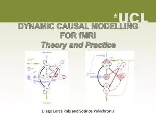
Dynamic Causal Modelling for fMRI. Rosie Coleman Philipp Schwartenbeck. Methods for dummies 2012/13 With thanks to Peter Zeidman & ' Ōiwi Parker-Jones. Outline. DCM: Theory Background Basis of DCM Hemodynamic model Neuronal Model Developments in DCM DCM: Practice

E N D
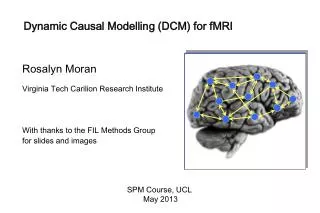
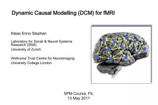
Dynamic Causal Modelling for fMRI Rosie Coleman Philipp Schwartenbeck Methods for dummies 2012/13 With thanks to Peter Zeidman & 'Ōiwi Parker-Jones
Outline • DCM: Theory • Background • Basis of DCM • Hemodynamic model • Neuronal Model • Developments in DCM • DCM: Practice • Experimental Design • Step-by-step guide
The connected brain “We can isolate processes occurring in the living organism and describe then in terms and laws of physico-chemistry. […] But when it comes to the properly ‘vital’ features, it is found that they are essentially problems of organisation, […] resulting from the interaction of an enormous number of highly complicated physico-chemical events.” (von Bertalanffy, 1950) “The functional role, played by any component (e.g., cortical area, sub-area, neuronal population or neuron) of the brain, is defined largely by its connections. Functional Specialisation is only meaningful in the context of functional integration and vice versa.” (Friston, 2003) “Yet, there does not seem to be a single area for which we are able to deduce its functional properties in a direct and causal fashion from its microstructural properties.” (Stephan, 2004)
Types of Connectivity • Anatomical connectivity • Anatomical layout of axons and synaptic connections • Which neural units interact directly with each other • E.g. DTI • Functional connectivity • Correlation among activity in different brain areas • Statistical dependencies between measured time series • Effective connectivity • Causal influence that one neuronal system exerts over another • At synaptic or neuronal population level
Effective Connectivity • Two basic implications • Effective connectivity is dynamic • i.e. activity- and time-dependent • That means influence of neuronal system on another changes with time and context • Effective connectivity includes interactions (nonlinearities)between neuronal systems • Models of connectivity need to rely on effective connectivity to be biologically plausible • Brain is dynamic • Current state of brain effects its state in the future • As sampling rate of measurement increases, data becomes more dynamic (PET -> fMRI –> MEEG) • Brain is nonlinear • Non-additive (interactions) effects like saturation, habituation,…
Methods based on effective connectivity • Structural Equation modelling • Multivariate analysis testing for influences among interacting variables • Time-series analysis • E.g. Granger Causality • Can dynamics of region A be predicted better using past values of region A and region B as opposed to using past values of region A alone • Methods based on linear regression analysis, e.g. • Psychophysical-Interaction analysis • Methods based on nonlinear dynamic models • Dynamic Causal Modelling (DCM)
Problems of other methods than DCM • Most methods do not allow to test for directionality/causality • Impossible to characterise by methods based on regression • Regarding inputs as stochastic (noise) • Idea of experiment is to change connectivity in a controlled way • Input therefore is not stochastic but experimentally controlled • Relying on hemodynamic response (BOLD-signal) • Definition of effective connectivity: influences of neuronal system • Transformation from neuronal activity to hemodynamic response has non-linear components • Not trivial to estimate to what degree the estimated coupling in the hemodynamic response was affected by transformation • Cf. David et al., 2008
Basis of DCM “The central idea behind dynamic causal modelling (DCM) is to treat the brain as a deterministic nonlinear dynamic system that is subject to inputs and produces outputs.” (Friston, 2003)
Brain as input-state-output system • Two types of inputs: • Influence on specific anatomical regions (nodes) • Modulation of coupling among regions (nodes) • E.g. visual input:
Brain as input-state-output system • Inputs: experimental manipulations • External input on brain, e.g. visual stimuli • Context, e.g. attention • State variables: neuronal activities in the brain • Outputs: electromagnetic or hemodynamic responses over brain regions • Measured in scanner
Hemodynamic “Forward” model • Effective connectivity: influence that one neuronal system exerts over another • Problem: neuronal activity not directly accessible in fMRI… • Hemodynamic “forward” model of how neuronal synaptic activity transformed into measured response • Key difference to other measurements of connectivity
Forward model • Neuronal dynamics (z) transformed into BOLD-signal (y) via hemodynamic response function (λ) • DCM: Usethisspecificmodeltoestimateparametersat neuronal level • Such thatmodelledandmeasured BOLD signalmaximallysimilar For details see Stephan et al., 2007…
What is DCM modelling? Forward model:
Neuronal model • Aim: model temporal evolution of set of neuronal states zt • Important: not interested in neuronal state itself, but its rate of change in time • Due to experimental perturbation in system • Expressed in differential equation: current state Intrinsic connectivity external input
General State Equation z: current state of system z2 z3 u: external input to system θ: intrinsic connectivity Z1
Neural State Equation in DCM • Example: attention to motion or colour of visual stimulus (Chawla, 1999) • Neural system consisting of: • 4 nodes (regions) • Connections • Within regions • Between regions • External input • Stimulus • Context Taken from: Stephan, 2004
Neural State Equation in DCM Problem: want to account for changes in connectivity due to input… • : change in neuralsystem • A: connectivity matrix if no input • Intrinsic coupling in absence of experimental perturbations • z: nodes (regions) • C: extrinsic influences of inputs on neuronal activity in regions • u: inputs
Neural State Equation in DCM • : change in neuralsystem • A: connectivity matrix if no input • Intrinsic coupling in absence of experimental perturbations • B: change in intrinsic coupling due to input • z: nodes (regions) • C: extrinsic influences of inputs on neuronal activity in regions • u: inputs Allowing for interactions between input and activity in region (i.e. nonlinearities)
Neural State Equation in DCM • Having established this neural state equation, we can now specify DCMs to look at: • Intrinsic coupling between regions (A matrix) • Changes in coupling due to external input (B matrix) • Usually most interesting • Direct influences of inputs on regions (C matrix)
Standard fMRI as special case of DCM • Btw: Assuming that B=[] and only allowing for connectivity within regions gives us… … a model for standard analysis of fMRI time-series (GLM for region-specific activation)…
Inference in DCM • Bayesian Inference • Relying on prior knowledge about connectivity parameters • Bayesian model selection to find model with highest model-evidence • Most likely connections & influences of inputs • Important: trade off between model fit and complexity (e.g., parameters in model) • Overfitting (i.e., explaining noise as well) if only aiming at best fit
Upgrades & more sophisticated DCMs • DCM10 • Intrinsic connectivity (A matrix) can be: • Coupling without any perturbation (at rest) • Coupling during average perturbation (during experiment) • Bilinear (as explained) or Nonlinear DCM (Stephan et al., 2008) • Including interactions with other units • Account more accurately for processes like attention, learning, … • Deterministic (as explained) or Stochastic DCM (Daunizeau et al., 2009) • Including noise, short-term variations in effective connectivity • One-state (as explained) or two-state DCM (Marreiros et al., 2008) • Splitting every z in inhibitory and excitatory neuronal population • Higher biological plausibility • All changes: http://tinyurl.com/bueuqae
Interim Summary • Dynamic Causal Modelling measures effective connectivity in the brain • Dynamic: capturing dependencies of brain regions over time • Causal: measuring effective connectivity (i.e., causal influence of one neuronal system over another) • Nonlinear: interactions between inputs and activity in regions • Hemodynamic “forward” model • Accounting for neuronal coupling (not coupling in BOLD-signal) • Allows to account for effective connectivity • Neuronal model • Express changes in neural states via parameters for • Intrinsic connectivity • Influence of inputs on connectivity • Influence of inputs on brain regions
Steps for conducting a DCM study on fMRI data… • Planning a DCM study • The example dataset • Identify your ROIs & extract the time series • Defining the model space • Model Estimation • Bayesian Model Selection/Model inference • Family level inference • Parameter inference • Group studies
Planning a DCM Study • DCM can be applied to most datasets analysed using a GLM. • BUT! there are certain parameters that can be optimised for a DCM study. • If you’re interested… Daunizeau, J., Preuschoff, K., Friston, K., & Stephan, K. (2011). Optimizing experimental design for comparing models of brain function. PLoS Computational Biology, 7(11)
Attention to Motion Dataset • Can be downloaded from the SPM website • Question: Why does attention cause a boost of activity on V5? • 4 Conditions: • Inputs to our models: • 1. Photic input to V1 • 2. Motion modulatory input acting on the coupling from V1→V5 • We know about these inputs, so they are the same in each model, and we do not need to model variations on where the inputs may enter the system because that is known. • The only unknown is the point at which attention modulates V5 activation. • As such, we are only going to look at two possible models.
MODEL 1 Attentionalmodulation of V1→V5 forward/bottom-up MODEL 2 Attentionalmodulation of SPM→V5 backward/ top-down
1. Extracting the time-series • Define your contrast (e.g. task vs. rest) and extract the time-series for the areas of interest. • The areas need to be the same for all subjects. • There needs to be significant activation in the areas that you extract. • For this reason, DCM is not appropriate for resting state studies • (NB: you can use stochastic DCM to model resting state – but this is computationally demanding. To read more about this see references at the end. Don’t ask me because I really can’t explain it to you.)
2. Defining the model space The models that you choose to define for your DCM depend largely on your hypotheses. • well-supported predictions • inferences on model structure → can define a small number of possible models. • no strong indication of network structure • inferences on connection strengths → may be useful to define all possible models. • Use anatomical and computational knowledge. • More models does NOT mean you must correct for multiple comparisons! • Number of models = where c = number of connections. • E.g. 4 areas, all connected bilinearly, with no diagonal connections = 8 connections = = 256 possible models.
At this stage, you can specify various options. • MODULATORY EFFECTS: bilinearvsnon-linear • STATES PER REGION: one vs. two • STOCHASTIC EFFECTS: yes vs. no • CENTRE INPUT: yes vs. no
3. Model Estimation • Fit your predicted model to the data. • The dotted lines represent the data, full lines represent the regions, blue being V1, green V5 and red SPC. • Bottom graph shows your parameter estimates.
Separate fitting of identical models for each subject Family Level Model Level Does the winning family differ by group/condition/performance? Does the winning model differ by group/condition/performance? Parameter Level Within Groups Between Groups parameter 1 > parameter 2 ? parameter > 0 ? Does connection strength vary by performance/symptoms/other variable? Connection from region A ->region B group 1 > group 2 ?
4. BMS & Model-Level Inference • Choose directory • Load all models for all subjects (must be estimated!) • Choose FFX or RFX – Multiple subjects with possibility for different models = RFX • Optional: • Define families • Compute BMA • Use ‘load model space’ to save time (this file is included in Attention to Motion dataset)
Winning Model! MODEL 1 Attentional modulation of V1→V5 forward/bottom-up
Modulatory Connections Intrinsic Connections
Separate fitting of identical models for each subject Family Level Model Level Does the winning family differ by group/condition/performance? Does the winning model differ by group/condition/performance? Parameter Level Within Groups Between Groups parameter 1 > parameter 2 ? parameter > 0 ? Connection from region A ->region B group 1 > group 2 ? Does connection strength vary by performance/symptoms/other variable?
5. Family-Level Inference • Often, there doesn’t appear to be one model that is an overwhelming ‘winner’ • In these circumstances, we can group similar models together to create families. • By sorting models into families with common characteristics, you can aggregate evidence. • We can then use these to pool model evidence and make inferences at the level of the family. Penny, W. D., Stephan, K. E., Daunizeau, J., Rosa, M. J., Friston, K. J., Schofield, T. M., & Leff, A. P. (2010). Comparing families of dynamic causal models. PLoSComputational Biology, 6(3)
Separate fitting of identical models for each subject Family Level Model Level Does the winning family differ by group/condition/performance? Does the winning model differ by group/condition/performance? Parameter Level Within Groups Between Groups parameter 1 > parameter 2 ? parameter > 0 ? Connection from region A ->region B group 1 > group 2 ? Does connection strength vary by performance/symptoms/other variable?
6. Parameter-Level Inference Parameter Level Within Groups Bayesian Model Averaging • Calculates the mean parameter values, weighted by the evidence for each model. • BMA uses a default of 10000 samples to create this average value. • BMA values therefore account for uncertainty in your data. parameter 1 > parameter 2 ? parameter > 0 ? Does connection strength vary by performance/symptoms/other variable? • BMA can be calculated on an individual subject, or at a group level. • Within a group (or on a single subject) you can use T-tests to compare connection strengths. • Can assess the relationship between connection strength and some linear variable e.g. performance, symptoms, age using regression analysis/correlation.
7. Group Studies Parameter Level Between Groups • DCM can be fruitful for investigating group differences. • E.g. patients vs. controls • Groups may differ in; • Winning model • Winning family • Connection values as defined using BMA Connection from region A ->region B group 1 > group 2 ? Seghier, M. L., Zeidman, P., Neufeld, N. H., Leff, A. P., & Price, C. J. (2010). Identifying abnormal connectivity in patients using dynamic causal modeling of FMRI responses. Frontiers in systems neuroscience, 4(August), 1–14.
connection strength vs. connection strength ← Network reconfiguration and working memory impairment in mesial temporal lobe epilepsy. Campoet al (2013) NeuroImage connection strength vs. performance ← ↙ ↑ connection strength – patients vs. controls Recent example of how you can use DCM to make inferences at the model, family, and parameter level.
Thank you for listening … and special thanks to Peter Zeidman & 'ŌiwiParker-Jones!