Download
1 / 29
290 likes | 602 Views
Dynamic Causal Modelling (DCM) for fMRI. Andre Marreiros. Wellcome Trust Centre for Neuroimaging University College London. Overview. Dynamic Causal Modelling of fMRI. Definitions & motivation. The neuronal model (bilinear dynamics) The Haemodynamic model. Estimation: Bayesian framework.

E N D
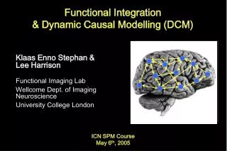
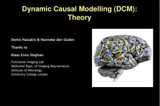
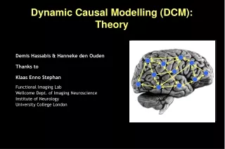
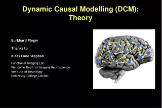
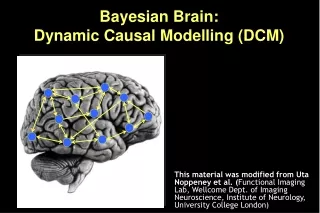
Dynamic Causal Modelling (DCM) for fMRI Andre Marreiros Wellcome Trust Centre for Neuroimaging University College London
Overview Dynamic Causal Modelling of fMRI Definitions & motivation • The neuronal model(bilinear dynamics) • The Haemodynamic model • Estimation: Bayesian framework • DCM latest Extensions
Principles of organisation Functional specialization Functional integration
Input u(t) c1 b23 neuronal states a12 activity z2(t) activity z3(t) activity z1(t) y y y BOLD Conceptual overview
State vector • Changes with time system represented by state variables • Rate of change of state vector • Interactions between elements • External inputs, u • System parameters Use differential equations to represent a neuronal system
DCM parameters = rate constants Generic solution to the ODEs in DCM: Decay function: Half-life:
z2 sa21t z1 Linear dynamics: 2 nodes z1 z2
Neurodynamics: 2 nodes with input u1 u2 u1 z1 z1 z2 z2 activity in z2 is coupled to z1 via coefficient a21
Neurodynamics: positive modulation u1 u1 u2 u2 z1 z1 z2 z2 index, not squared modulatory input u2 activity through the coupling a21
Neurodynamics: reciprocal connections u1 u1 u2 u2 z1 z1 z2 z2 reciprocal connection disclosed by u2
Haemodynamics: reciprocal connections u1 BOLD (without noise) u2 h1 z1 BOLD (without noise) h2 z2 blue: neuronal activity red: bold response h(u,θ) represents the BOLD response (balloon model) to input
Haemodynamics: reciprocal connections u1 BOLD with Noise added u2 y1 z1 BOLD with Noise added y2 z2 blue: neuronal activity red: bold response y represents simulated observation of BOLD response, i.e. includes noise
Bilinear state equation in DCM for fMRI modulation of connectivity state vector direct inputs state changes externalinputs connectivity n regions m drv inputs m mod inputs
The haemodynamic “Balloon” model 5 haemodynamic parameters:
z λ y Conceptual overview Neuronal state equation The bilinear model effective connectivity modulation of connectivity Input u(t) direct inputs c1 b23 integration neuronal states a12 activity z2(t) activity z3(t) activity z1(t) haemodynamic model y y y BOLD Friston et al. 2003,NeuroImage
State space Model Model inversion using Expectation-maximization DCM roadmap Neuronal dynamics Haemodynamics Priors Posterior densities of parameters fMRI data Model comparison
Estimation: Bayesian framework • Models of • Haemodynamics in a single region • Neuronal interactions • Constraints on • Haemodynamic parameters • Connections likelihood term prior posterior Bayesian estimation
stimulus function u Overview:parameter estimation neuronal state equation • Specify model (neuronal and haemodynamic level) • Make it an observation model by adding measurement errore and confounds X (e.g. drift). • Bayesian parameter estimation using expectation-maximization. • Result:(Normal) posterior parameter distributions, given by mean ηθ|y and Covariance Cθ|y. parameters hidden states state equation ηθ|y observation model modeled BOLD response
Parameter estimation: an example Input coupling, c1 Simulated response u1 z1 Forward coupling, a21 z2 Prior density Posterior density true values
Inference about DCM parameters:single-subject analysis • Bayesian parameter estimation in DCM: Gaussian assumptions about the posterior distributions of the parameters • Quantify the probability that a parameter (or contrast of parameters cT ηθ|y) is above a chosen threshold γ: ηθ|y
Pitt & Miyung (2002), TICS Model comparison and selection Given competing hypotheses, which model is the best?
Attention to motion in the visual system We used this model to assess the site of attention modulation during visual motion processing in an fMRI paradigm reported by Büchel & Friston. Attention Time [s] ? SPC Photic • - fixation only • observe static dots + photic V1 • - observe moving dots + motion V5 • task on moving dots + attention V5 + parietal cortex V5 V1 Motion Friston et al. 2003,NeuroImage
Model 2:attentional modulationof SPC→V5 SPC V1 V5 Attention Photic 0.55 0.86 0.75 1.42 0.89 -0.02 0.56 Motion Comparison of two simple models Model 1:attentional modulationof V1→V5 Photic SPC 0.85 0.70 0.84 1.36 V1 -0.02 0.57 V5 Motion 0.23 Attention Bayesian model selection: Model 1 better than model 2 → Decision for model 1: in this experiment, attention primarily modulates V1→V5
Extension I: Slice timing model • potential timing problem in DCM: temporal shift between regional time series because of multi-slice acqisition 2 slice acquisition 1 visualinput • Solution: • Modelling of (known) slice timing of each area. • Slice timing extension now allows for any slice timing differences! • Long TRs (> 2 sec) no longer a limitation. • (Kiebel et al., 2007)
¶ x = + u ( AB ) x Cu ¶ t é ù é ù L EE EI E A - - x A A e e e 0 11 11 1 N 1 ê ú ê ú IE II I - x A A e e 0 0 ê ú ê ú 11 11 1 ê ú ê ú M = = M O M A x ( t ) ê ú ê ú EE EI E A - - x A A ê ú e 0 e e ê ú N 1 NN NN N ê ú ê ú L IE II I - x A A 0 0 e e ë û ë û NN NN N Extension II: Two-state model Single-state DCM Two-state DCM input Extrinsic (between-region) coupling Intrinsic (within-region) coupling
DCM for Büchel & Friston Attention - BCW Attention b - Intr Example: Two-state Model Comparison - FWD Attention
Extension III: Nonlinear DCM for fMRI nonlinear DCM bilinear DCM u2 u2 u1 u1 Bilinear state equation Nonlinear state equation Here DCM can model activity-dependent changes in connectivity; how connections are enabled or gated by activity in one or more areas.
Extension III: Nonlinear DCM for fMRI Can V5 activity during attention to motion be explained by allowing activity in SPC to modulate the V1-to-V5 connection? attention . 0.19 (100%) The posterior density of indicates that this gating existed with 97.4% confidence. (The D matrix encodes which of the n neural units gate which connections in the system) SPC 0.03 (100%) 0.01 (97.4%) 1.65 (100%) visual stimulation V1 V5 0.04 (100%) motion
Conclusions Dynamic Causal Modelling (DCM) of fMRI is mechanistic model that is informed by anatomical and physiological principles. DCM uses a deterministic differential equation to model neuro-dynamics (represented by matrices A,B and C) DCM uses a Bayesian framework to estimate model parameters DCM provides an observation model for neuroimaging data, e.g. fMRI, M/EEG DCM is not model or modality specific (Models will change and the method extended to other modalities e.g. ERPs)