Download
1 / 37
370 likes | 565 Views
Tradeoffs Among Life History Traits There are tradeoffs among different life history traits and among the costs associated with them. Without tradeoffs the logical direction for species to evolve would be more of everything: more offspring, larger offspring

E N D
Tradeoffs Among Life History Traits There are tradeoffs among different life history traits and among the costs associated with them. Without tradeoffs the logical direction for species to evolve would be more of everything: more offspring, larger offspring size, better survivorship and longer life. The hypothesis of reproductive cost explains the tradeoffs between increased reproduction and other aspects of the life history. By extension, it also applies to other possible tradeoffs. Tradeoffs may occur in the behaviour, physiology, and strategies of individuals, but may also involve balances between parents and offspring, called `inter-generational', or occur at the population level.
The idea of tradeoffs as an important life history argument may be only 20 – 30 years old, but it is not new. From R.A. Fisher's classic book The Genetical Theory of Natural Selection (1930): "It would be instructive to know not only by what physiological mechanisms a just apportionment is made between the nutriment devoted to the gonads and that devoted to the rest of the parental organism, but also what circumstances in the life-history and environment would render profitable the diversion of a greater or lesser share of the available resources towards reproduction."
Compromises may occur among: Individual traits: a) current reproduction (measured as mx) b) future reproduction (residual reproductive value, Vx+1) c) parental survival (measured by lx or px) d) parental growth e) parental condition Inter-generation traits: f) offspring growth g) offspring condition h) offspring survival Population level traits: i) number of offspring j) size of offspring
All strategies are compromises between lx and mx. More explicitly – the foundation of life history theory is the hypothesis of reproductive cost. Any increase in present reproduction (at least in an iteroparous species) is associated with a decrease in future (or alternatively residual) reproductive value, i.e. the expected contribution to future generations resulting from all future bouts of reproduction. The decrease could be either reduced fecundity in the future, or reduced survivorship. This can be represented in an equation for reproductive value having two components: current reproduction and the value of future reproduction (Vx+1) in a population which is changing in size.
It is this negative correlation between reproductive effort in the present and the value of future reproduction which makes the optimization of timing and intensity of reproductive effort possible. If there weren't a negative correlation, then species would maximize both current and future reproduction, as well as beginning as early as possible and lasting as long through life as possible. The idea of reproductive cost is explained using the principle of allocation: An organism has a limited set of basic functions or needs which must be met: these functions are usually classed as maintenance, growth and reproduction.
Maintenance refers to baseline metabolism plus costs borne • to ensure survival, e.g. water regulation, resistance to predation, competition or disease, etc. It does not include any component of increase. • 2. Growth refers to the energetic cost of increase. • 3. Reproduction refers to costs of producing gametes, of • acquiring mates (including development of displays, • behaviours, etc.), of bearing the young, and of parental care. • There are energetic costs associated with each function, and clearly energy allocated to one function is not available for the others. Thus there are reciprocal adjustments among functions, and evolution should favor adjustments which maximize fitness.
Variations in patterns of allocation among these functions may be genetic or phenotypic, and may occur in many factors important to fitness, including age of first reproduction, temporal pattern of reproduction (the shape of the mx curve; semelparity versus iteroparity, and the size of mx. We will explore data that examines evidence of tradeoffs and adaptations evident in many of these variables.
Semelparity versus Iteroparity It’s almost Shakespearean… Whether to reproduce only once (i.e. semelparity or big-bang reproduction), or whether to reproduce more moderately but repeatedly (i.e. iteroparity). Reproducing early, and using the big- bang approach, the organism need not worry about possible effects on adult survivorship. Caution can be “thrown to the winds”. The generation time, G, will be considerably shortened, and R0 can be increased. This should clearly increase 'r'. However, even if every litter were somewhat smaller, the iteroparous species can have many such litters, and a much larger number of offspring (R0) over a life cycle. The answer (which is the better strategy) is not clear.
A comparison of strategies is part of Cole's (1954) classic paper, and comes to what, at the outset, seems to be a shocking conclusion. Here are the parameters of Cole’s comparison: 1) Assume that the semelparous species has perfect survivorship to age 1 year, then reproduces, producing a litter of size b. 2) Assume that the iteroparous species has perfect survivorship, not only until it begins reproducing at age 1, but also thereafter; it produces a litter of size b annually. Now compare the population growth...
First the semelparous species. The exponential growth model: Nt = N0 ert if t = 1 year, and each female has a litter of size b, then the growth equation can be re-written: Nt/N0 = er = b or rs = ln (b) The calculations for the iteroparous species involve another infinite sum, with the approximate result that: ri = ln (b+1)
Cole's way of stating this comparative result is clear and concise: “for an annual species, the absolute gain in intrinsic population growth which could be achieved by changing to the perennial reproductive habit would be exactly equivalent to adding one individual to the average litter size.”
Not only that, but the gain, logically, is a function of litter size and the age of first reproduction, which aren't considered in this basic comparison. The gain from changing to iteroparity (when the litter size of the semelparous species is equal) increases both with delay in first reproduction (i.e. increasing ) and with decreasing litter size. Consider why… If it takes one extra in the litter for a semelparous species to keep up, that represents a bigger proportional increase in reproductive effort when litter size is small than when it's large. Now consider the effects of changing . The general idea can best be seen by comparing population size over time in semelparous and iteroparous populations.
First in the comparison that produced the original result: Time 0 1 2 3 4 Semelparity 1 b b2 b3 b4 Iteroparity 1 b+1 b2 +2b+1 b3+3b2+3b+1 (b+1)4 Now, what happens if were 2… Time 0 1 2 3 4 Semelparity 1 b b2 Iteroparity 1 b+1 2b+1 b2+4b+1
If alpha increased from 1 to 5 for both the iteroparous and semelparous species being compared, then by the time grandchildren are born in the semelparous species, the iteroparous parent will have produced offspring at ages 6,7,8 and 9, each time with a litter of size b. That's clearly a bigger advantage than accrued when alpha was 1. Cole showed the general result in a graph:
Most semelparous species tend to have short pre-reproductive periods. That minimizes the advantage that might be gained by becoming iteroparous. A few examples make the basic point. Annual plants (many weeds) and almost all insects complete their life cycles in a single year, and most which do not complete life cycles in 2 years instead (e.g. biennial plants such as weedy thistles, teasel, onions, garlic). Semelparous species also typically have very large litter sizes. Many produce 106 eggs or more, e.g. Musca domestica, the common housefly, oysters, or the salmon.
The problem can also be approached from the opposite point of view. It is clearly advantageous, from an evolutionary view, to increase the intrinsic rate of increase 'r', 'all else being equal'. A change in 'r' could result from becoming iteroparous while maintaining litter size, or from an increase in the semelparous litter size. Since either change could be equally effective, we can look at the change in semelparous litter size required to achieve the same 'r' as would be reached by switching to iteroparity while just maintaining litter size. Since Cole worked it out so nicely, I’ll use it even though it is an animal example…
The change in litter size required can be dramatic. Take the lowly tapeworm as an example: The approximate daily litter size of the mature tapeworm is 100,000 eggs. Including larval development time, the maturation time, or alpha, is approximately 100 days.
If the tapeworm were to become indefinitely iteroparous, we find that the equivalent semelparous litter size to achieve the same growth rate would be about 800,000 (or an increase in litter size by a factor of 8). The species is not, of course, indefinitely iteroparous, and the required semelparous litter (or litter size factor) size is not quite so large. There are real situations which suggest a considerable advantage (in an evolutionary sense) to iteroparity.
Effects of age of first reproduction There is an approximately inverse relationship between rmax and generation time (see the table below), which, if perfect, would have indicated a constant R0 over a wide variety of taxa. Generation time is also related to body size, both in the maturation time and in the interval between births. Both of these relationships are demonstrated in plots in the text and below. It's clear that instantaneous rates of increase would increase in organisms with shorter generation times among whom R0 is constant (and, thus, inversely related to body mass). Even though the simple formula (ln R0/G) calculates only an approximate r, it is apparent that a smaller generation time G would increase the rate of increase.
Values for rmax, the generation time G, and their product as an indication of potential growth rate . Taxon Species rmax G r x G Bacteria E. coli 60. .014 .84 Protazoa Paramecium aurelia 1.24 .40 .508 P. caudatum .94 .30 .282 Insecta Tribolium confusum 12 80. 9.60 Calandra oryzae .11 58. 6.38 Eurostis hilleri .01 110. 1.1 Magicicada septendecim .001 6050. 6.05 Mammalia Rattus norvegicus .015 150. 2.25 Microsus agrestis .013 171. 2.22 Canis domesticus .009 1000. 9.0 Homo sapiens .0003 7000. 2.1
There are allometric relationships between many physical and life history variables that have been measured. If we take body mass, M, as the base variable, these relationships seem to take the form of power laws. The general form, taking Y as the dummy variable standing in for the many others, is: Y = Y0Mb Normally these relationships are plotted after a log transform, since they are then linear: log Y = log Y0 + blog M The b values seem always to be multiples of 0.25. For heart rate versus mass, b = -0.25 For mass and basal metabolic rate b = 0.75 For mass and resource use b = 0.75
In birds, mass and both life span and reproductive maturity scale with a b = 0.25. There are many more examples, and in sum they have led to an attempt to formulate a general theory: It is called the Metabolic Theory of Ecology, and begins with the scaling ideas you’ve just seen, then adds well-recognized temperature-dependence of biological processes. The theory then claims that life history characteristics are determined by metabolic processes whose rates are determined by scaling and absolute temperature. These ideas are the subject of ongoing controversy. Whatever the bases, you should now recognize that large-bodied plants and animals will have low r values, slow development, and different life history compromises than small ones.
Example 1: The California condor
Tradeoff between Reproductive Effort and Survivorship in the California Condor The California Condor is an endangered species very close to extinction. Recent release of captive-raised condors suggests there may be hope for the species. In 1985 there were less than 10 breeding pairs remaining in the wild; four years later (1989) this condor had gone extinct in the wild. In 1987, anticipating this, the San Diego Zoo initiated a captive breeding program. Almost two decades before extinction in the wild, David Mertz (1971) predicted that the species would be virtually impossible to save, based both on the disappearance of its native habitat as southern California became increasingly urbanized, and on its demography.
The condor does not exhibit the demographic pattern usually • associated with birds, i.e. type II diagonal survivorship curve. • Instead, • it is very long-lived and has a very low reproductive rate. • The condor does not become reproductively mature until • at least 5 years old, and may not mature for twice that time. • California condors produce only a single egg every other • year, though most condors produce annual broods of 2 eggs • and some produce only a single egg each year. • While the mean lifespan is high, there is significant pre- • reproductive mortality, somewhat concentrated in the first • year.
From these basic facts, we can construct a hypothetical life table for the condor, and look for factors in it which may explain the decline of the population. • We can, for purposes of calculations using this life table, • lump all pre-reproductive mortality and call survivorship • from birth to age b. • 2. Given the long lifespan, we can reasonably assume that adult proportional survivorship is uniform through the reproductive span. That proportional survivorship we'll call p. • 3. Since only a single egg is produced every other year, if =5, we assign these eggs to the odd years. Since only half of these eggs will be female, the mx we put in the life table for years with reproduction is 1/2.
Now we can construct the life table… Age x lx mx lxmx 0... - 0 0 5 b .5 b/2 6 bp 0 0 7 bp2 .5 bp2/2 8 bp3 0 0 9 bp4 .5 bp4/2 ... Calculations for this life table: The net replacement rate turns out to be the sum of a power series, which, when p < 1, can be simplified to a formula: R0 = lxmx = b/2 (1 + p2 + p4 + ...) = b/[2(1-p2)]
Now, to maintain the population, R0 must equal 1 (we'll assume, given the low mx and observation of declining numbers that we don't need to consider the potential for growth). Then: 1 = b/[2(1-p2)] b = 2(1-p2) or 1-b/2 = p2 If b ~ 0 (very severe pre-reproductive mortality) then adult mortality cannot be tolerated, p = 1 (adults must remain immortal). If juvenile survivorship is extremely high, b = 1, note that adult survivorship must still be high, with a p = .7071. If about half of juveniles survive to reproductive maturity, then adult proportional survivorship must be .86.
The solid lines are the observed demography of the condor, and the dashed lines represent the demography if condors re-nest the year after a nesting failure. In actuality, the re-nesting rate is only about 50% of nestling mortality.
Since we're interested only in the narrow range 0 < b, p < 1, we can closely approximate the mathematical parabola by a straight line over that range. That isocline for R0 = 1 divides the plot into two regions. Below that line R0 < 1, and the population declines; above the isocline R0 > 1, and the population grows. Increase is possible only with very high adult survivorship, and even with perfect survivorship the population grows by only 15% per year due to the extremely low reproductive rate. Realistically the survivorship of mature adults must almost certainly be higher than that for inexperienced juveniles, i.e. p > b. Insert a diagonal line where p = b; only points to the left of the diagonal are now realistic values for survivorships. With this assumption the minimum adult survivorship to maintain the population is p = .78.
The isocline for R0 = 1 is relatively 'shallow'. R0 is relatively insensitive to changes in prereproductive survivorship; only slight changes occur with relatively large shifts in b. However, R0 is exquisitely sensitive to changes in p.
Mertz (1971) made two key points based on these observations: 1) Even slight hunting or poaching of adult birds, could take a tenuously stable population into a relatively rapid decline. 2) The differing sensitivity also suggests an explanation for a key management difficulty. Any disturbance of nesting females will cause the nesting female to leave her eggs for a period sufficient to frequently allow cooling and mortality of the embryos. That behaviour - taking off rather than defending the nest - is what might be expected when juvenile (or egg) mortality can be tolerated (in a quantitative sense) more than adult mortality. This is the first indication of a tradeoff .
3) It might seem that this strategy is based solely on maintenance of a high lx, but there is also pressure on mx. The rate of egg production must remain very close to one egg every other year; it is not tolerable to miss producing an egg. Any decline in mx must be made up by an increase in lx to maintain R0 = 1. With the already extreme demands on survivorship, there is no room left in the demographic pattern to enhance adult survivorship. • What about long maturation time? It might seem that if birds simply started laying eggs earlier, that net replacement rates would climb, and reduce the pressure on survivorship. The condor is altricial; most altricial birds have an alpha of approximately 2, far lower than the minimum of 5 for the California condor.
There is little effect from changing when the population is stable or growing. However, when the population is in decline (due to an insufficient p) a decrease in only accelerates the decline, because the survivorship schedule shifts from b (low sensitivity) to that insufficient p earlier.
The dashed lines are what would happen if the condor shifted to age 4. For growing populations the dashed lines lie below the solid ones; equal growth (R0) could be achieved with slightly lower p and b. However, when the population is declining the dashed lines lie above the solid ones. All these facts make it apparent that game managers attempting to protect the endangered California condor were fighting a losing battle from the start. All they could do was attempt to prevent as much non-natural mortality as possible to protect p, and exert what little influence such managers have over the expanding destruction of native habitat in southern California.
It seems likely that only continuing release of birds from the remaining zoo-raised population will keep the California condor present in the natural world over the long term. However, there are now (April 2009) 172 free condors in California and Arizona (data retrieved from Wikipedia, so open to question). The conservation goal is a total of at least 150 birds in each of two disjunct populations, with at least 15 breeding pairs in each. That would lead to the species being downgraded to “threatened” from “endangered”.