Download
1 / 81
810 likes | 835 Views
This seminar explores the nearest neighbor problem, classical nearest neighbor methods, and efficient search techniques in high dimensions. Topics include KD-trees, bucketing methods, and locality sensitive hashing.

E N D
Nearest Neighbor Search in High Dimensions Seminar in Algorithms and Geometry Mica Arie-Nachimson and Daniel Glasner April 2009
Talk Outline • Nearest neighbor problem • Motivation • Classical nearest neighbor methods • KD-trees • Efficient search in high dimensions • Bucketing method • Locality Sensitive Hashing • Conclusion Main Results Indyk and Motwani, 1998 Gionis, Indyk and Motwani, 1999
Nearest Neighbor Problem • Input: A set P of points in Rd (or any metric space). • Output: Given a query point q, find the point p* in P which is closest to q. q p*
What is it good for? Many things! Examples: • Optical Character Recognition • Spell Checking • Computer Vision • DNA sequencing • Data compression
What is it good for? Many things! Examples: • Optical Character Recognition • Spell Checking • Computer Vision • DNA sequencing • Data compression 2 query 1 2 2 3 7 7 2 2 3 8 4 Feature space
What is it good for? Many things! Examples: • Optical Character Recognition • Spell Checking • Computer Vision • DNA sequencing • Data compression query abaut shout bat abate scout about boat able Feature space
What is it good for? Many things! Examples: • Optical Character Recognition • Spell Checking • Computer Vision • DNA sequencing • Data compression And many more…
Approximate Nearest Neighbor -NN • Input: A set P of points in Rd (or any metric space). • Given a query point q, let: • p* point in P closest to q • r* the distance ||p*-q|| • Output: Some point p’ with distance at most r*(1+) q r* p*
Approximate Nearest Neighbor -NN • Input: A set P of points in Rd (or any metric space). • Given a query point q, let: • p* point in P closest to q • r* the distance ||p*-q|| • Output: Some point p’ with distance at most r*(1+) ·r*(1+) q r* p* ·r*(1+)
Approximate vs. ExactNearest Neighbor • Many applications give similar results with approximate NN • Example from Computer Vision
Retiling Slide from Lihi Zelnik-Manor
Approximate NNS ~0.6 sec Exact NNS ~27 sec Slide from Lihi Zelnik-Manor
Solution Method • Input: A set P of n points in Rd. • Method: Construct a data structure to answer nearest neighbor queries • Complexity • Preprocessing: space and time to construct the data structure • Query: time to return answer
Solution Method • Naïve approach: • Preprocessing O(nd) • Query time O(nd) • Reasonable requirements: • Preprocessing time and space poly(nd). • Query time sublinear in n.
Talk Outline • Nearest neighbor problem • Motivation • Classical nearest neighbor methods • KD-trees • Efficient search in high dimensions • Bucketing method • Locality Sensitive Hashing • Conclusion
Classical nearest neighbor methods • Tree structures • kd-trees • Vornoi Diagrams • Preprocessing poly(n), exp(d) • Query log(n), exp(d) • Difficult problem in high dimensions • The solutions still work, but are exp(d)…
KD-tree • d=1 (binary search tree) 5 20 7 8 10 12 13 15 18 7,8,10,12 13,15,18 13,15 18 7,8 10,12 7, 8 10, 12 13, 15 18
KD-tree • d=1 (binary search tree) 5 20 7 8 10 12 13 15 18 query 17 7,8,10,12 13,15,18 13,15 18 7,8 10,12 min dist = 1 7, 8 10, 12 13, 15 18
KD-tree • d=1 (binary search tree) 5 20 7 8 10 12 13 15 18 query 16 7,8,10,12 13,15,18 13,15 18 7,8 10,12 min dist = 2 min dist = 1 7, 8 10, 12 13, 15 18
KD-tree • d>1: alternate between dimensions • Example: d=2 (12,5) (6,8) (17,4) (23,2) (20,10) (9,9) (1,6) (12,5) (6,8) (1,6) (9,9) (17,4) (23,2) (20,10) x y x
KD-tree • d>1: alternate between dimensions • Example: d=2 x x y x
x x y x KD-tree: complexity • Preprocessing O(nd) • Query • O(logn) if points are randomly distributed • w.c. O(kn1-1/k) almost linear when n close to k • Need to search the whole tree
Talk Outline • Nearest neighbor problem • Motivation • Classical nearest neighbor methods • KD-trees • Efficient search in high dimensions • Bucketing method • Locality Sensitive Hashing • Conclusion
Sublinear solutions 2 Not counting logn factors Linear in d Solve -NN by reduction
r-PLEBPoint Location in Equal Balls • Given n balls of radius r, for every query q, find a ball that it resides in, if exists. • If doesn’t reside in any ball return NO. Return p1 p1
r-PLEBPoint Location in Equal Balls • Given n balls of radius r, for every query q, find a ball that it resides in, if exists. • If doesn’t reside in any ball return NO. Return NO
Reduction from -NN to r-PLEB • The two problems are connected • r-PLEB is like a decision problem for -NN
Reduction from -NN to r-PLEB • The two problems are connected • r-PLEB is like a decision problem for -NN
Reduction from -NN to r-PLEB • The two problems are connected • r-PLEB is like a decision problem for -NN
Reduction from -NN to r-PLEBNaïve Approach • Set R=proportion between largest dist and smallest dist of 2 points • Define r={(1+)0, (1+)1,…,R} • For each ri construct ri-PLEB • Given q, find the smallest r* which gives a YES • Use binary search to find r*
r3-PLEB r2-PLEB r1-PLEB Reduction from -NN to r-PLEBNaïve Approach • Set R=proportion between largest dist and smallest dist of 2 points • Define r={(1+)0, (1+)1,…,R} • For each ri construct ri-PLEB • Given q, find the smallest ri which gives a YES • Use binary search
Reduction from -NN to r-PLEBNaïve Approach • Correctness • Stopped at ri=(1+)k • ri+1=(1+)k+1 (1+)k · r* · (1+)k+1 r3-PLEB r2-PLEB r1-PLEB
Reduction from -NN to r-PLEBNaïve Approach Reduction overhead: • Space: O(log1+R) r-PLEB constructions • Size of {(1+)0, (1+)1,…,R} is log1+R • Query: O(loglog1+R) calls to r-PLEB Dependency on R
Reduction from -NN to r-PLEBBetter Approach • Set rmed as the radius which gives n/2 connected components (C.C) Har-Peled 2001
Reduction from -NN to r-PLEBBetter Approach • Set rmed as the radius which gives n/2 connected components (C.C)
Reduction from -NN to r-PLEBBetter Approach • Set rmed as the radius which gives n/2 connected components (C.C) • Set rtop= 4nrmedlogn/ rtop rmed
Reduction from -NN to r-PLEBBetter Approach • If q2 B(pi,rmed) and q2 B(pi,rtop), set R=rtop/rmed and perform binary search on r={(1+)0, (1+)1,…,R} • R independent of input points • If q2 B(pi,rmed) q2 B(pi,rtop) 8 i then q is “far away” • Enough to choose one point from each C.C and continue recursively with these points (accumulating error · 1+/3) • If q2 B(pi,rmed) for some i then continue recursively on the C.C. rmed
Reduction from -NN to r-PLEBBetter Approach • If q2 B(pi,rmed) and q2 B(pi,rtop), set R=rtop/rmed and perform binary search on r={(1+)0, (1+)1,…,R} • R independent of input points • If q2 B(pi,rmed) q2 B(pi,rtop) 8 i then q is “far away” • Enough to choose one point from each C.C and continue recursively with these points (accumulating error · 1+/3) • If q2 B(pi,rmed) for some i then continue recursively on the C.C. rtop
Reduction from -NN to r-PLEBBetter Approach • If q2 B(pi,rmed) and q2 B(pi,rtop), set R=rtop/rmed and perform binary search on r={(1+)0, (1+)1,…,R} • R independent of input points • If q2 B(pi,rmed) q2 B(pi,rtop) 8 i then q is “far away” • Enough to choose one point from each C.C and continue recursively with these points (accumulating error · 1+/3) • If q2 B(pi,rmed) for some i then continue recursively on the C.C. rtop
Reduction from -NN to r-PLEBBetter Approach • If q2 B(pi,rmed) and q2 B(pi,rtop), set R=rtop/rmed and perform binary search on r={(1+)0, (1+)1,…,R} • R independent of input points • If q2 B(pi,rmed) q2 B(pi,rtop) 8 i then q is “far away” • Enough to choose one point from each C.C and continue recursively with these points (accumulating error · 1+/3) • If q2 B(pi,rmed) for some i then continue recursively on the C.C. rmed
Reduction from -NN to r-PLEBBetter Approach • If q2 B(pi,rmed) and q2 B(pi,rtop), set R=rtop/rmed and perform binary search on r={(1+)0, (1+)1,…,R} • R independent of input points • If q2 B(pi,rmed) q2 B(pi,rtop) 8 i then q is “far away” • Enough to choose one point from each C.C and continue recursively with these points (accumulating error · 1+/3) • If q2 B(pi,rmed) for some i then continue recursively on the C.C. rmed
Reduction from -NN to r-PLEBBetter Approach • If q2 B(pi,rmed) and q2 B(pi,rtop), set R=rtop/rmed and perform binary search on r={(1+)0, (1+)1,…,R} • R independent of input points • If q2 B(pi,rmed) q2 B(pi,rtop) 8 i then q is “far away” • Enough to choose one point from each C.C and continue recursively with these points (accumulating error · 1+/3) • If q2 B(pi,rmed) for some i then continue recursively on the C.C. rmed
Reduction from -NN to r-PLEBBetter Approach • If q2 B(pi,rmed) and q2 B(pi,rtop), set R=rtop/rmed and perform binary search on r={(1+)0, (1+)1,…,R} • R independent of input points • If q2 B(pi,rmed) q2 B(pi,rtop) 8 i then q is “far away” • Enough to choose one point from each C.C and continue recursively with these points (accumulating error · 1+/3) • If q2 B(pi,rmed) for some i then continue recursively on the C.C. rmed
Reduction from -NN to r-PLEBBetter Approach • If q2 B(pi,rmed) and q2 B(pi,rtop), set R=rtop/rmed and perform binary search on r={(1+)0, (1+)1,…,R} • R independent of input points • If q2 B(pi,rmed) q2 B(pi,rtop) 8 i then q is “far away” • Enough to choose one point from each C.C and continue recursively with these points (accumulating error · 1+/3) • If q2 B(pi,rmed) for some i then continue recursively on the C.C. O(loglogR)=O(log(n/)) 2 + half of the points Complexity overhead: how many r-PLEB queries? Total: O(logn)
(r,)-PLEBPoint Location in Equal Balls • Given n balls of radius r, for query q: • If q resides in a ball of radius r, return the ball. • If q doesn’t reside in any ball, return NO. • If q resides only in the “border” of a ball, return either the ball or NO. Return p1 p1
(r,)-PLEBPoint Location in Equal Balls • Given n balls of radius r, for query q: • If q resides in a ball of radius r, return the ball. • If q doesn’t reside in any ball, return NO. • If q resides only in the “border” of a ball, return either the ball or NO. Return NO
(r,)-PLEBPoint Location in Equal Balls • Given n balls of radius r, for query q: • If q resides in a ball of radius r, return the ball. • If q doesn’t reside in any ball, return NO. • If q resides only in the “border” of a ball, return either the ball or NO. Return YES or NO