Download
1 / 34
400 likes | 1.08k Views
Algorithms for Nearest Neighbor Search. Piotr Indyk MIT. Nearest Neighbor Search. Given: a set P of n points in R d Goal: a data structure, which given a query point q , finds the nearest neighbor p of q in P. p. q. Outline of this talk. Variants Motivation

E N D
Algorithms for Nearest Neighbor Search Piotr Indyk MIT
Nearest Neighbor Search • Given: a set P of n points in Rd • Goal: a data structure, which given a query point q, finds the nearest neighborp of q in P p q
Outline of this talk • Variants • Motivation • Main memory algorithms: • quadtrees • kd-trees • Locality Sensitive Hashing • Secondary storage algorithms: • R-tree (and its variants) • VA-file
Variants of nearest neighbor • Near neighbor (range search): find one/all points in P within distance r from q • Spatial join: given two sets P,Q, find all pairs p in P, q in Q, such that p is within distance r from q • Approximate near neighbor: find one/all points p’ in P, whose distance to q is at most (1+e) times the distance from q to its nearest neighbor
Motivation Depends on the value of d: • low d: graphics, vision, GIS, etc • high d: • similarity search in databases (text, images etc) • finding pairs of similar objects (e.g., copyright violation detection) • useful subroutine for clustering
Algorithms • Main memory (Computational Geometry) • linear scan • tree-based: • quadtree • kd-tree • hashing-based: Locality-Sensitive Hashing • Secondary storage (Databases) • R-tree (and numerous variants) • Vector Approximation File (VA-file)
Quadtree • Simplest spatial structure on Earth !
Quadtree ctd. • Split the space into 2d equal subsquares • Repeat until done: • only one pixel left • only one point left • only a few points left • Variants: • split only one dimension at a time • k-d-trees (in a moment)
Range search • Near neighbor (range search): • put the root on the stack • repeat • pop the next node T from the stack • for each child C of T: • if C is a leaf, examine point(s) in C • if C intersects with the ball of radius r around q, add C to the stack
Nearest neighbor • Start range search with r = • Whenever a point is found, update r • Only investigate nodes with respect to current r
Quadtree ctd. • Simple data structure • Versatile, easy to implement • So why doesn’t this talk end here ? • Empty spaces: if the points form sparse clouds, it takes a while to reach them • Space exponential in dimension • Time exponential in dimension, e.g., points on the hypercube
K-d-trees [Bentley’75] • Main ideas: • only one-dimensional splits • instead of splitting in the middle, choose the split “carefully” (many variations) • near(est) neighbor queries: as for quadtrees • Advantages: • no (or less) empty spaces • only linear space • Exponential query time still possible
Exponential query time • What does it mean exactly ? • Unless we do something really stupid, query time is at most dn • Therefore, the actual query time is Min[ dn, exponential(d) ] • This is still quite bad though, when the dimension is around 20-30 • Unfortunately, it seems inevitable (both in theory and practice)
Approximate nearest neighbor • Can do it using (augmented) k-d trees, by interrupting search earlier [Arya et al’94] • Still exponential time (in the worst case)! • Try a different approach: • for exact queries, we can use binary search trees or hashing • can we adapt hashing to nearest neighbor search ?
Locality-Sensitive Hashing [Indyk-Motwani’98] • Hash functions are locality-sensitive, if, for a random hash random function h, for any pair of points p,q we have: • Pr[h(p)=h(q)] is “high” if p is “close” to q • Pr[h(p)=h(q)] is “low” if p is”far” from q
Do such functions exist ? • Consider the hypercube, i.e., • points from {0,1}d • Hamming distance D(p,q)= # positions on which p and q differ • Define hash function h by choosing a set I of k random coordinates, and setting h(p) = projection of p on I
Example • Take • d=10, p=0101110010 • k=2, I={2,5} • Then h(p)=11
h’s are locality-sensitive • Pr[h(p)=h(q)]=(1-D(p,q)/d)k • We can vary the probability by changing k Pr k=1 Pr k=2 distance distance
How can we use LSH ? • Choose several h1..hl • Initialize a hash array for each hi • Store each point p in the bucket hi(p) of the i-th hash array, i=1...l • In order to answer query q • for each i=1..l, retrieve points in a bucket hi(q) • return the closest point found
What does this algorithm do ? • By proper choice of parameters k and l, we can make, for any p, the probability that hi(p)=hi(q) for some i look like this: • Can control: • Position of the slope • How steep it is distance
The LSH algorithm • Therefore, we can solve (approximately) the near neighbor problem with given parameter r • Worst-case analysis guarantees dn1/(1+e) query time • Practical evaluation indicates much better behavior [GIM’99,HGI’00,Buh’00,BT’00] • Drawbacks: • works best for Hamming distance (although can be generalized to Euclidean space) • requires radius r to be fixed in advance
Secondary storage • Seek time same as time needed to transfer hundreds of KBs • Grouping the data is crucial • Different approach required: • in main memory, any reduction in the number of inspected points was good • on disk, this is notthe case !
Disk-based algorithms • R-tree [Guttman’84] • departing point for many variations • over 600 citations ! (according to CiteSeer) • “optimistic” approach: try to answer queries in logarithmic time • Vector Approximation File [WSB’98] • “pessimistic” approach: if we need to scan the whole data set, we better do it fast • LSH works also on disk
R-tree • “Bottom-up” approach (k-d-tree was “top-down”) : • Start with a set of points/rectangles • Partition the set into groups of small cardinality • For each group, find minimum rectangle containing objects from this group • Repeat
R-tree ctd. • Advantages: • Supports near(est) neighbor search (similar as before) • Works for points and rectangles • Avoids empty spaces • Many variants: X-tree, SS-tree, SR-tree etc • Works well for low dimensions • Not so great for high dimensions
VA-file [Weber, Schek, Blott’98] • Approach: • In high-dimensional spaces, all tree-based indexing structures examine large fraction of leaves • If we need to visit so many nodes anyway, it is better to scan the whole data set and avoid performing seeks altogether • 1 seek = transfer of few hundred KB
VA-file ctd. • Natural question: how to speed-up linear scan ? • Answer: use approximation • Use only i bits per dimension (and speed-up the scan by a factor of 32/i) • Identify all points which could be returned as an answer • Verify the points using original data set
Time to sum up • “Curse of dimensionality” is indeed a curse • In main memory, we can perform sublinear-time search using trees or hashing • In secondary storage, linear scan is pretty much all we can do (for high dim) • Personal thought: if linear search is all we can do, we are not doing too well…. • Maybe it is time to buy a few GB of RAM • ..but at the end everything depends on your data set
Resources • Surveys: • Berchtold & Keim: • http://www.informatik.unihalle.de/~keim/PS/ICDE00.pdf • Theodoridis: • http://dias.cti.gr/~ytheod/research/ADBIS/handouts.pdf • Agarwal et al (range searching): • http://www.cs.duke.edu/~pankaj/papers.html
Resources • Source code: http://dias.cti.gr/~ytheod/research/indexing/ http://www.cs.sunysb.edu/~algorith/major_section/1.6.shtml • References: see surveys plus very recent • [Buh’00,BT’00]: J. Buhler et al: http://www.cs.washington.edu/homes/jbuhler/ • [HGI’00]: Haveliwala et al: http://theory.lcs.mit.edu/~indyk/webdb.ps
Contact • If you have any question, feel free to e-mail me at indyk@theory.lcs.mit.edu • Thank you !