Download
1 / 47
500 likes | 538 Views
Nearest Neighbor & Information Retrieval Search. Artificial Intelligence CMSC 25000 January 29, 2004. Agenda. Machine learning: Introduction Nearest neighbor techniques Applications: Robotic motion, Credit rating Information retrieval search Efficient implementations:

E N D
Nearest Neighbor &Information Retrieval Search Artificial Intelligence CMSC 25000 January 29, 2004
Agenda • Machine learning: Introduction • Nearest neighbor techniques • Applications: Robotic motion, Credit rating • Information retrieval search • Efficient implementations: • k-d trees, parallelism • Extensions: K-nearest neighbor • Limitations: • Distance, dimensions, & irrelevant attributes
Nearest Neighbor • Memory- or case- based learning • Supervised method: Training • Record labeled instances and feature-value vectors • For each new, unlabeled instance • Identify “nearest” labeled instance • Assign same label • Consistency heuristic: Assume that a property is the same as that of the nearest reference case.
Nearest Neighbor Example • Problem: Robot arm motion • Difficult to model analytically • Kinematic equations • Relate joint angles and manipulator positions • Dynamics equations • Relate motor torques to joint angles • Difficult to achieve good results modeling robotic arms or human arm • Many factors & measurements
Nearest Neighbor Example • Solution: • Move robot arm around • Record parameters and trajectory segment • Table: torques, positions,velocities, squared velocities, velocity products, accelerations • To follow a new path: • Break into segments • Find closest segments in table • Get those torques (interpolate as necessary)
Nearest Neighbor Example • Issue: Big table • First time with new trajectory • “Closest” isn’t close • Table is sparse - few entries • Solution: Practice • As attempt trajectory, fill in more of table • After few attempts, very close
Nearest Neighbor Example II • Credit Rating: • Classifier: Good / Poor • Features: • L = # late payments/yr; • R = Income/Expenses Name L R G/P A 0 1.2 G B 25 0.4 P C 5 0.7 G D 20 0.8 P E 30 0.85 P F 11 1.2 G G 7 1.15 G H 15 0.8 P
Nearest Neighbor Example II Name L R G/P A 0 1.2 G A F B 25 0.4 P 1 G R E C 5 0.7 G H D C D 20 0.8 P E 30 0.85 P B F 11 1.2 G G 7 1.15 G 10 20 30 L H 15 0.8 P
Nearest Neighbor Example II Name L R G/P I 6 1.15 G A F K J 22 0.45 P 1 I G ?? E K 15 1.2 D H R C J B Distance Measure: Sqrt ((L1-L2)^2 + [sqrt(10)*(R1-R2)]^2)) - Scaled distance 10 20 30 L
Efficient Implementations • Classification cost: • Find nearest neighbor: O(n) • Compute distance between unknown and all instances • Compare distances • Problematic for large data sets • Alternative: • Use binary search to reduce to O(log n)
Roadmap • Problem: • Matching Topics and Documents • Methods: • Classic: Vector Space Model • Challenge I: Beyond literal matching • Expansion Strategies • Challenge II: Authoritative source • Page Rank • Hubs & Authorities
Matching Topics and Documents • Two main perspectives: • Pre-defined, fixed, finite topics: • “Text Classification” • Arbitrary topics, typically defined by statement of information need (aka query) • “Information Retrieval”
Three Steps to IR • Three phases: • Indexing: Build collection of document representations • Query construction: • Convert query text to vector • Retrieval: • Compute similarity between query and doc representation • Return closest match
Matching Topics and Documents • Documents are “about” some topic(s) • Question: Evidence of “aboutness”? • Words !! • Possibly also meta-data in documents • Tags, etc • Model encodes how words capture topic • E.g. “Bag of words” model, Boolean matching • What information is captured? • How is similarity computed?
Models for Retrieval and Classification • Plethora of models are used • Here: • Vector Space Model
Vector Space Information Retrieval • Task: • Document collection • Query specifies information need: free text • Relevance judgments: 0/1 for all docs • Word evidence: Bag of words • No ordering information
Vector Space Model Tv Program Computer Two documents: computer program, tv program Query: computer program : matches 1 st doc: exact: distance=2 vs 0 educational program: matches both equally: distance=1
Vector Space Model • Represent documents and queries as • Vectors of term-based features • Features: tied to occurrence of terms in collection • E.g. • Solution 1: Binary features: t=1 if present, 0 otherwise • Similiarity: number of terms in common • Dot product
Question • What’s wrong with this?
Vector Space Model II • Problem: Not all terms equally interesting • E.g. the vs dog vs Levow • Solution: Replace binary term features with weights • Document collection: term-by-document matrix • View as vector in multidimensional space • Nearby vectors are related • Normalize for vector length
Vector Similarity Computation • Similarity = Dot product • Normalization: • Normalize weights in advance • Normalize post-hoc
Term Weighting • “Aboutness” • To what degree is this term what document is about? • Within document measure • Term frequency (tf): # occurrences of t in doc j • “Specificity” • How surprised are you to see this term? • Collection frequency • Inverse document frequency (idf):
Term Selection & Formation • Selection: • Some terms are truly useless • Too frequent, no content • E.g. the, a, and,… • Stop words: ignore such terms altogether • Creation: • Too many surface forms for same concepts • E.g. inflections of words: verb conjugations, plural • Stem terms: treat all forms as same underlying
Key Issue • All approaches operate on term matching • If a synonym, rather than original term, is used, approach fails • Develop more robust techniques • Match “concept” rather than term • Expansion approaches • Add in related terms to enhance matching • Mapping techniques • Associate terms to concepts • Aspect models, stemming
Expansion Techniques • Can apply to query or document • Thesaurus expansion • Use linguistic resource – thesaurus, WordNet – to add synonyms/related terms • Feedback expansion • Add terms that “should have appeared” • User interaction • Direct or relevance feedback • Automatic pseudo relevance feedback
Query Refinement • Typical queries very short, ambiguous • Cat: animal/Unix command • Add more terms to disambiguate, improve • Relevance feedback • Retrieve with original queries • Present results • Ask user to tag relevant/non-relevant • “push” toward relevant vectors, away from nr • β+γ=1 (0.75,0.25); r: rel docs, s: non-rel docs • “Roccio” expansion formula
Compression Techniques • Reduce surface term variation to concepts • Stemming • Map inflectional variants to root • E.g. see, sees, seen, saw -> see • Crucial for highly inflected languages – Czech, Arabic • Aspect models • Matrix representations typically very sparse • Reduce dimensionality to small # key aspects • Mapping contextually similar terms together • Latent semantic analysis
Authoritative Sources • Based on vector space alone, what would you expect to get searching for “search engine”? • Would you expect to get Google?
Issue Text isn’t always best indicator of content Example: • “search engine” • Text search -> review of search engines • Term doesn’t appear on search engine pages • Term probably appears on many pages that point to many search engines
Hubs & Authorities • Not all sites are created equal • Finding “better” sites • Question: What defines a good site? • Authoritative • Not just content, but connections! • One that many other sites think is good • Site that is pointed to by many other sites • Authority
Conferring Authority • Authorities rarely link to each other • Competition • Hubs: • Relevant sites point to prominent sites on topic • Often not prominent themselves • Professional or amateur • Good Hubs Good Authorities
Computing HITS • Finding Hubs and Authorities • Two steps: • Sampling: • Find potential authorities • Weight-propagation: • Iteratively estimate best hubs and authorities
Sampling • Identify potential hubs and authorities • Connected subsections of web • Select root set with standard text query • Construct base set: • All nodes pointed to by root set • All nodes that point to root set • Drop within-domain links • 1000-5000 pages
Weight-propagation • Weights: • Authority weight: • Hub weight: • All weights are relative • Updating: • Converges • Pages with high x: good authorities; y: good hubs
Google’s PageRank • Identifies authorities • Important pages are those pointed to by many other pages • Better pointers, higher rank • Ranks search results • t:page pointing to A; C(t): number of outbound links • d:damping measure • Actual ranking on logarithmic scale • Iterate
Contrasts • Internal links • Large sites carry more weight • If well-designed • H&A ignores site-internals • Outbound links explicitly penalized • Lots of tweaks….
Web Search • Search by content • Vector space model • Word-based representation • “Aboutness” and “Surprise” • Enhancing matches • Simple learning model • Search by structure • Authorities identified by link structure of web • Hubs confer authority
Efficient Implementation: K-D Trees • Divide instances into sets based on features • Binary branching: E.g. > value • 2^d leaves with d split path = n • d= O(log n) • To split cases into sets, • If there is one element in the set, stop • Otherwise pick a feature to split on • Find average position of two middle objects on that dimension • Split remaining objects based on average position • Recursively split subsets
R > 0.825? L > 17.5? L > 9 ? R > 0.6? R > 0.75? R > 1.175 ? R > 1.025 ? K-D Trees: Classification Yes No No Yes Yes No No Yes No Yes No No Yes Yes Poor Good Good Poor Good Good Poor Good
Efficient Implementation:Parallel Hardware • Classification cost: • # distance computations • Const time if O(n) processors • Cost of finding closest • Compute pairwise minimum, successively • O(log n) time
Nearest Neighbor: Issues • Prediction can be expensive if many features • Affected by classification, feature noise • One entry can change prediction • Definition of distance metric • How to combine different features • Different types, ranges of values • Sensitive to feature selection
Nearest Neighbor Analysis • Problem: • Ambiguous labeling, Training Noise • Solution: • K-nearest neighbors • Not just single nearest instance • Compare to K nearest neighbors • Label according to majority of K • What should K be? • Often 3, can train as well
Nearest Neighbor: Analysis • Issue: • What is a good distance metric? • How should features be combined? • Strategy: • (Typically weighted) Euclidean distance • Feature scaling: Normalization • Good starting point: • (Feature - Feature_mean)/Feature_standard_deviation • Rescales all values - Centered on 0 with std_dev 1
Nearest Neighbor: Analysis • Issue: • What features should we use? • E.g. Credit rating: Many possible features • Tax bracket, debt burden, retirement savings, etc.. • Nearest neighbor uses ALL • Irrelevant feature(s) could mislead • Fundamental problem with nearest neighbor
Nearest Neighbor: Advantages • Fast training: • Just record feature vector - output value set • Can model wide variety of functions • Complex decision boundaries • Weak inductive bias • Very generally applicable
Summary • Machine learning: • Acquire function from input features to value • Based on prior training instances • Supervised vs Unsupervised learning • Classification and Regression • Inductive bias: • Representation of function to learn • Complexity, Generalization, & Validation
Summary: Nearest Neighbor • Nearest neighbor: • Training: record input vectors + output value • Prediction: closest training instance to new data • Efficient implementations • Pros: fast training, very general, little bias • Cons: distance metric (scaling), sensitivity to noise & extraneous features