Download
1 / 33
330 likes | 337 Views
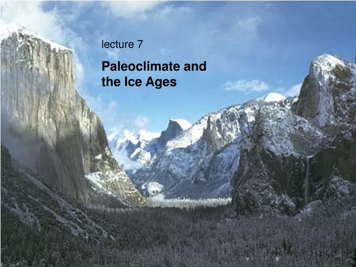
lecture 7 Paleoclimate and the Ice Ages. Ruth Valley Glacier Alaska --The glacier occupying Yosemite Valley probably looked similar.

E N D
lecture 7 Paleoclimate and the Ice Ages
Ruth Valley Glacier Alaska--The glacier occupying Yosemite Valley probably looked similar.
Over the past 2 million years, the earth has had ice sheets which have varied in size, causing alternations between ice ages and interglacial periods. This entire time period is known as the Pleistocene.
Glaciers also exist at high altitudes in the tropics. The annual accumulation of snow, which provides climate information at yearly resolution, is clearly visible in this photograph of a tropical glacier.
Key definitions cryosphere snow cover glacier ice sheet
Where are the ice sheets in the present-day climate? In the northern hemisphere, Greenland is covered by an enormous ice sheet which is a few kilometers thick and more than five times larger than the state of California in area. If this ice sheet were to melt, global sea level would rise by about 7 meters. This is all that remains of the huge ice sheets that covered North America and Eurasia during the last glacial maximum, about 20,000 years ago.
In the southern hemisphere, the Antarctic continent is covered with an even larger ice sheet. The Antarctic continent is about 25% larger than the United States. If this ice sheet were to melt entirely, global sea level would rise by about 70 meters. About 80% of the planet’s freshwater is locked up in this ice sheet. The Greenland ice sheet contains about 9% of the planet’s freshwater, with the remainder being contained mostly in lakes and mountain glaciers.
The extent of the northern hemisphere ice sheets at the last glacial maximum. The expansion of these ice sheets resulted in a sea level approximately 130 meters lower than today’s.
Deformation of the land surface, such as glacial moraines, are evidence of ice sheet extent
Because of the lowered sea level, the coastlines during the last ice age differed significantly from today’s. North America was connected to Eurasia by a land bridge where the Bering strait is today, and the Mediterranean basin was cut off from the Atlantic.
It is possible to reconstruct an approximate chronology of the ice ages by measuring the oxygen isotopes in ocean sediment cores. As marine organisms perish, their skeletons are deposited on the bottom of the sea floor. The layers of deposited skeletons provide information about climate.
OXYGEN ISOTOPES The chemical elements are often found in more than one form. The number of protons in the atomic nucleus is constant for any given element, but the number of neutrons in the nucleus can vary. The chemical behavior of isotopes of the same element is very similar, the main difference being their weight. Oxygen primarily comes in two isotopes: Oxygen 16 and Oxygen 18. Oxygen 18 has two extra neutrons, making it about 10% heavier than Oxygen 16.
ICE VOLUME EFFECT ON OXYGEN ISOTOPES The ratio of the heavier to the lighter oxygen isotope varies in the ambient seawater because of the variations in total ice volume. The water molecules containing the heavier isotope are less likely evaporate and be incorporated into the ice sheet. So as total ice volume increases, the ocean becomes increasingly enriched in the heavier isotope of oxygen.
TEMPERATURE EFFECT ON OXYGEN ISOTOPES When temperatures are colder, the organisms incorporate more of the heavier isotope of oxygen into their skeletons. Measuring the ratio of the heavier to the lighter oxygen isotope in the skeletons therefore indicates how warm the water was when the organism was alive.
OXYGEN ISOTOPE SIGNATURE IN SEDIMENT CORES So when ocean temperatures are cold and ice volume is large, the skeletons should be enriched in the heavier isotope. Presumably temperature and ice volume are tightly correlated, so an examination of the oxygen isotope record in ocean sediment cores gives us a clear picture of when the ice ages occurred.
This is the oxygen isotope record from the Pacific Ocean off the coast of South America. It reveals that the ice ages occurred approximately once every 100,000 years.
The orbits of the planets are ellipses (from Kepler’s law). If you take any two points (called foci) in space, you can define an ellipse as the collection of points whose combined distance to the two points is a constant. In the case of the planets’ orbit, the sun is at one of the two foci of the elliptical orbit.
The point in the orbit when the a planet is closest to the sun is called perihelion. The point when the planet is furthest from the sun is called the aphelion. In the case of earth’s orbit, perihelion occurs in early January, while aphelion occurs in early July. The planet gets more sunshine at perihelion, and less at aphelion, because of the inverse square law.
The planet orbits faster when it is closest to the sun. So perihelion is the point in the orbit when the planet is traveling the fastest. This is why our calendar months have irregular lengths. Pope Gregory XIII hired some astronomers to create the Gregorian calendar (1582) to guarantee the solstices and equinoxes would always fall on the 21st of Dec, Mar, Jun, and Sep.
The eccentricity of the earth’s orbit varies between 0 an 0.06 with a period of about 100,000 years and 400,000 years. This variation is due to the gravitational pull of other planets.
The axis about which the earth rotates is tilted relative to the plane of the earth’s orbit. This tilt, called obliquity, is the reason why our planet has seasons. Currently the earth’s obliquity is 23.5 degrees. If the obliquity were 0 (i.e. no tilt), the northern hemisphere would get about the same amount of sunshine all year round.
The tilt of a spinning object can vary; earth is no exception. The obliquity of the earth varies between about 22 and 24 degrees with a period of about 41,000 years.
The direction of the earth’s spin axis also precesses. This means that the earth’s spin axis traces out a circle. Like obliquity, precession occurs on very long time scales. It takes about 20,000 years for the spin axis to trace out a circle once.
The situation now. Aphelion occurs in early July and coincides with northern hemisphere summer. The situation about 10,000 years ago in the opposite phase of the earth’s precessional cycle. Aphelion occurs in early January and coincides with southern hemisphere summer.
Summary: how orbital variations affect sunshine Obliquity When obliquity is high, seasonality is enhanced. In mid and high latitudes, more sunshine comes in summer, and less comes in winter. Averaged over the whole year, the high latitudes receive more sunshine, and the low latitudes receive less. Precession When perihelion occurs at summer solstice, the contrast between summer and winter is enhanced. When perihelion occurs at winter solstice, seasonality is weakened. Precession has little effect on annual mean sunshine. Eccentricity Changes in the eccentricity of the earth’s orbit have very little effect on the annual mean sunshine anywhere. However, they do have a large impact on the amplitude of the precessional cycle. If the earth’s orbit is very eccentric, the timing of perihelion in the calendar year becomes more critical.
The periodicities associated with variations in the earth’s orbit are dominant in chronologies of ice volume!
It is possible to quantify how much variability is associated with every time scale using a statistical technique called spectrum analysis. We can apply this technique to the ice volume time series, and measure how much variability occurs at the orbital time scales.
Spectrum of ice volume history Milutin Milankovitch (1879-1958) Note the clear peaks in the spectrum at the time scales associated with orbital variability. In fact over 95% of the variability occurs at these time scales. The idea that orbital variations might be responsible for climate variability is called the Milankovitch theory of climate.
So how might orbital variations cause ice ages? One idea is that since the ice sheets melt the most in the summertime, the sunshine during this time of year might be important for determining ice volume. But exactly how orbital variability is translated into the huge observed climate changes remains one of the major unsolved problems of climate. Any satisfactory explanation will probably involve the dynamics of the ice sheets themselves.
Another major unsolved problem: why do the greenhouse gases vary in phase with the ice ages?