Download
1 / 33
330 likes | 343 Views
Fluorescent Indicators. Martin Thomas, Cairn Research Ltd. Optical Measurements Are Sensitive!. Electric current 1A = 6.25 x 10 18 electrons/sec Squid axon voltage clamp 1mA 10 16 charges/sec Microelectrode voltage clamp 10uA 10 14 charges/sec, down to approx

E N D
Fluorescent Indicators Martin Thomas, Cairn Research Ltd
Optical Measurements Are Sensitive! • Electric current 1A = 6.25 x 10¹⁸ electrons/sec • Squid axon voltage clamp 1mA 1016 charges/sec • Microelectrode voltage clamp 10uA 1014 charges/sec, down to approx 1nA 1010 charges/sec • Patch clamp 1pA 107 charges/sec • Optical Recording Photomultipliers and electron-multiplying CCD cameras can detect single photons, but we need a lot to get good images - tradeoff between spatial and time resolution
Optical Units Radiant Power • Watt (W) • Lumen (lm) Radiant Intensity • Watts / Steradian (W/sr) • Lumens / Steradian (candela) Illumination Intensity • Lux (lm m-2) • Footcandle (lm ft-2) At 555nm: 1W 680 lm 2.8x10¹⁸ photons sec-1
Fluorescence Fluorescence is is the absorption of light by a molecule, to form a short-lived excited state, followed by re-emission of light at a longer wavelength. A crib for becoming an instant expert: FLIM Fluorescence Lifetime IMaging FRET Fluorescence Resonant Energy Transfer FISH Fluorescence In Situ Hybridisation TIRF Total Internal Reflection Fluorescence FRAP Fluorescence Recovery After Photobleaching
Fluorescence Fluorescence is is the absorption of light by a molecule, to form a short-lived excited state, followed by re-emission of light at a longer wavelength. A crib for becoming an instant expert: FLIM Fluorescence Lifetime IMaging FRET Fluorescence Resonant Energy Transfer FISH Fluorescence In Situ Hybridisation TIRF Total Internal Reflection Fluorescence FRAP Fluorescence Recovery After Photobleaching FLAF Four Letter Acronym Fluorescence
Indicator structures (stolen from Roger Tsien)
Ca Indicator Spectra Fura2 EX spectra measured at 510nm EM, EM spectra measured at 340nm EX Ca bound Ca bound Ca free Indo1 Absorption (=EX?) spectra, EM spectra measured at 338nm EX Ca bound Ca free EX spectra dotted, EM spectra continuous, data from Invitrogen website
Na and pH Indicator Spectra SBFI EX spectra measured at 505nm EM, EM spectra measured at 340nm EX Na bound Na free BCECF EX spectra measured at 535nm EM, EM spectra measured at 480nm EX pH 5.2 pH 9.0 EX spectra dotted, EM spectra continuous, data from Invitrogen website
Fura8 from AAT-BioquestExcitation spectrum shifted to longer wavelengthsSo no need for UV-transmitting opticsBut seems more susceptible to photobleaching than Fura2
But the affinity of most indicators is too highto record transients properly! Slow Timescale Fast Timescale Endothelial cells plus ATP Hepatocytes plus flash-released IP3 Ogden et al (1995), Eur J Physiol 429, 587-591
Fluorescence Quantification Ca + IFREE = CaI (at equilibrium) KD = [Ca][IFREE]/[CaI], so [Ca] = KD[CaI]/[IFREE], or [Ca] = KD[CaI]/([ITOTAL] - [CaI]) If only CaI is fluorescent, then we can write: [Ca] = KDF/(FMAX - F) where FMAX is the fluorescence at saturating [Ca], i.e. [CaI] = [ITOTAL] If IFREE is also fluorescent, the relation becomes: [Ca] = KD(F - FMIN)/(FMAX - F) where FMIN is the fluorescence at zero [Ca], i.e. [IFREE] = [ITOTAL] A similar derivation for ratiometric quantification gives: [Ca] = KD x C(R - RMIN)/(RMAX - R) where C is is the relative change in fluorescence between zero and saturating [Ca] at the denominator wavelength of the ratio (see Grynkiewicz, Poenie and Tsien, 1985, J. Biol. Chem 260 p3440 for full derivation) For both quantification methods, BEWARE of buffering and saturation effects, which can significantly alter the amplitude and time course of the recorded signals.
Ratiometric Measurement • There must be a change in the shape (not just the amplitude) of the spectrum, so not possible for all indicators • Corrects for changes in indicator concentration and excitation light intensity • Easier quantification, as RMAX will be a known constant on a given experimental setup, whereas for nonratio indicators FMAX needs to be determined for each experiment • Can utilise changes in either excitation spectrum or emission spectrum • Detection of changes in emission spectrum is somewhat easier (use two detectors) • Detection of of changes in excitation spectrum requires sequential measurements at different wavelengths (e.g. use a monochromator) • A versatile measurement system should be able to handle both methods • May be possible with either method to use more than one indicator at the same time (if their spectra are sufficiently different)
Ratio change on K+ perfusion: movement artefacts on the 340nm and 380nm traces don’t show up on the ratio (vertical location of 340 and 380nm traces is arbitrary)
Loading Indicators Into Cells • Indicator needs to be membrane-impermeant in order to remain in the cell, but how do we put it there? • Microinjection can work well for large cells, but increasingly difficult for smaller cells. • Shotgun approach using coated gold beads can also work well (e.g. for tissue slices). Other membrane disruptive techniques such as electroporation may also be possible. • Can introduce polymeric (dextran linked) forms for cells that tend to expel small foreign molecules (e.g. plants). • Ester loading can work well for smaller cells; esterified forms are membrane permeant, and so can enter cell, then are hydrolysed to the active free (membrane-impermeant) forms by internal esterases. But internal compartments other than cytosol may also be loaded, depending on location of the esterases. • Genetic expression of a protein-based indicator is potentially very attractive, as expression can be targeted to specific cell compartments and the cells come ready-loaded. But problems here include time and effort to make the constructs, and generally more limited signal range than for chemically synthesised indicators. • In ALL CASES the presence of the indicator itself (e.g. buffering effects), as well as the means of its introduction, may disturb what you are trying to measure, so do remember this when planning experiments (e.g. use several different concentrations).
Filters and Dichroic Mirrors Transmission spectra for FM-143 filter set • Specialist coatings permit filters with almost any optical profile to be created
Luminous Intensity distribution curve High pressure Arc Lamps Arc Profile: Luminous intensity variation along lamp axis 75W lamp < 1mm
Mercury Arc : Arc Lamp Emission Spectra Xenon Arc :
High Intensity LEDs Blue wavelengths now especially powerful, but more power in the green would still be useful. Available wavelengths now down to 340nm (Fura2 excitation!) Lower spectrum is of a “white” lamp – actually blue with a phosphor.
Diffraction Grating Diffractive maxima occur at angles where the path length differences are an integral number of wavelengths. Thus longer wavelengths are diffracted at greater angles.
Monochromator Operation • Image of input slit formed at exit slit • Triangular bandpass profile • Optics must be matched to rest of optical system to maximise throughput
Detection Systems • PHOTOMULTIPLIERS: Cheap, fast, sensitive, can use adjustable diaphragm to determine field of view, can easily record data in same acquisition system as e.g. electrical data. Why not buy one or two to use alongside your expensive CCD camera? • PHOTODIODES: More background noise than photomultipliers, so not suitable for weak signals. Avalanche photodiodes (APDs) are better in this respect, but still inferior. However, photodiodes do have a higher quantum (i.e. detection) efficiency, so may be better for strong signals, where photon noise dominates. • CCD CAMERAS: More expensive, generally slower and more limited signal range, but give nice pictures for journal covers. 3D deconvolution in software can give reasonable depth resolution, but you need to record a vertical stack of images in order to to this. Cameras and software now much improved over earlier systems. • LASER SCANNING CONFOCAL: Unlike the above methods, out-of-focus light is rejected, allowing true vertical sectioning. Potentially much more detail, but tradeoff is longer acquisition time for a full image, although e.g. linescan mode can be fast. Range of usable dyes restricted by availability/cost of appropriate lasers. Two-photon systems potentially even better, but at a price. • NIPKOW DISC CONFOCAL: Scans multiple points on the specimen simultaneously, and images onto a CCD camera. Nice idea in principle, also gives nice pictures, but depth resolution is poorer. One problem seems to be that the optimum hole pattern in the spinning disc depends on the microscope objective, so a compromise here.
Photodetector QE Dotted lines show how response can be extended into the UV if the device has a quartz instead of glass window.
The “Cairnfocal” DMD-Based Confocal Microscope Attaches to the sideport of a fluorescence microscope The nonconjugate side images from the DMD's“off” pixels Light from DMD collected at 24 degrees focusses “normally” onto the cameras 62 is the DMD 66 and 66' are the conjugate and nonconjugate cameras 86 and 86' are the excitation light sources (generally just use 86)
Noise on Optical Signals • Detector will contribute noise, but this will be a constant amount, although it can vary widely between different types of detector. • Optical signals are inherently noisy because of statistical variation in arrival times of individual photons – this is termed shot noise. • Shot noise increases with the square root of the signal level. Therefore stronger signals are also noisier, and the signal-to-noise ratio increases only with the square root of the signal level, rather than linearly as one might have expected. • But there may be considerable scope for increasing the optical signal, as collection efficiency increases with the square of the numerical aperture (NA) of the system. • Can also increase illumination intensity of course, but there are practical limits (e.g. photobleaching). • Since noise sources are uncorrelated, the overall noise level is the square root of the sum of the squares of the individual components, so the total noise level is determined primarily by the largest one (more so than if they added linearly). • For weak signals, detector noise may dominate, so low noise here is important, e.g. photomultipliers, image intensifiers. • For stronger signals, shot noise is more likely to dominate, favouring use of more efficient (higher QE) detectors, e.g. avalanche photodiodes, back-thinned CCD chips. • Latest CCD cameras with “on chip multiplication” may offer high QE AND low detector noise, but the statistical nature of the multiplication is expected to increase the effective shot noise by 2, so even this is not a perfect solution!