Download
1 / 25
250 likes | 479 Views
Continuous probability distributions. Uniform probability distribution (ASW, section 6.1) Normal probability distribution (ASW, section 6.2) Table – Appendix B and inside front cover Excel – Appendix 6.2

E N D
Continuous probability distributions Uniform probability distribution (ASW, section 6.1) Normal probability distribution (ASW, section 6.2) Table – Appendix B and inside front cover Excel – Appendix 6.2 Bring the text to class on Wednesday, October 1. We will be using Table 1 of Appendix B of ASW. Notes for October 1, 2008
Probability density function • For a continuous random variable x, the probability that x takes on a specific value is zero. As a result, probabilities for values of x are assigned across an interval of values of x. The probability function f(x) that is used to assign these probabilities is termed the probability density function. • If a variable x has probability density function f(x), the probability that x takes on values between a and b is the area under the graph of f(x) that lies between a and b (or the integral of f(x) over the range a to b).
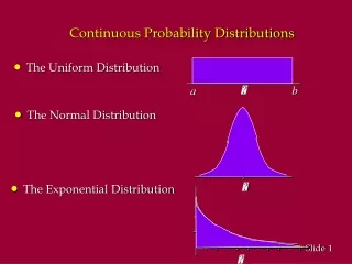
Uniform probability distribution (ASW, 226) • This is a distribution where the probability density function f(x) has the same value across all the values of x for which it is non-zero.
If x represents the variable being considered, the distribution has density f(x) = 1/(b – a) over the range from a to b and density of 0 elsewhere. Diagram of a uniform probability distribution a b f(x) 1/(b-a) x
Example – cost of travel Suppose a firm reimburses employees at the rate of 40 cents per kilometre when an employee uses his or her own automobile for company travel. Over the past years, the number of kilometres reimbursed in this manner has been between 100,000 and 150,000. The probability distribution of anticipated annual travel costs for the firm is considered to be a uniform distribution over this range. At the lower bound of 100,000 km., the total cost would be $40,000 and at the upper bound of 150,000 km., the total cost would be $60,000. Since travel is not anticipated to be less than 100,000 km. nor greater than 150,000 km., cost is zero outside the lower and upper bound.
Uniform probability distribution for travel example Let x be the anticipated total cost of annual travel for the firm in thousands of dollars. Then the uniform probability distribution is:
Let x represents the total anticipated annual travel costs in thousands of dollars, the distribution has density f(x) = 1/(60 - 40) = 1/20 over the range from 40 to 60and density of 0 elsewhere. Uniform probability distribution of total expected travel cost for the firm 40 60 f(x) 1/20 x Travel cost in thousands of dollars
f(x) 1/20 x 40 60 Travel costs Area of the distribution Note that the total area under the density function f(x) between 40 and 60 equals 1. Area = height x length = (1/20) x (60–40) = (1/20) x 20 = 1 and this equals the probability that some value within the range from 40 to 60 occurs.
f(x) 1/20 x 40 50 60 Travel costs Area and probability over an interval What is the probability that travel costs are between 40 and 50? Area under the curve between 40 and 50 = height x length = (1/20) x (50–40) = (1/20) x 10 = 0.5 and this is the required probability.
Expected value and variance for a uniform probability distribution For the travel cost example: E(x) = (40 + 60)/2 = 50 Var(x) = (60–40)2/12 = 33.333 Standard deviation of x is the square root of 33.333 or 5.774
Firm’s anticipated travel costs If the uniform distribution applies, then the firm might predict that travel costs will be $50,000 annually (the mean or expected value). However, there is variability in anticipated costs, with the standard deviation being $5,774. The probability that travel costs are within one standard deviation of the mean of $50,000 turns out to be 0.5774. This is the area under the line between 50,000 - 5,774 = 44,226 and 50,000 + 5,774 = 55,774. This is a distance of 11,548. The area under the line is (11,548/20,000) = 0. 5774. Note that the area under the curve within two standard deviations of the mean is the whole distribution.
Features of a continuous probability distribution ASW (228) • For a continuous probability distribution, the probability for the random variable must be defined over an interval, not at a single value of the variable. • The probability that the random variable takes on values within an interval is the area under the curve of the density function f(x) across that interval. (Or it equals the integral of f(x) from the lower to upper bounds of the interval). • Also note that the total area under the curve of the density function equals one. • Most continuous distributions do not have the linear or straight line characteristic of the uniform distribution, but will be nonlinear or curved. Tables of these distributions are often available. These tables give the required areas or probabilities.
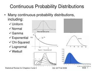
Normal probability distribution The normal probability distribution is the most common and important of the continuous probability distributions used in statistical and econometric work. Other names for the normal distribution are the bell curve, since it has a sort of bell shape, and the Gaussian distribution, after Gauss, who is considered to be the first to have described and used the distribution.
Formula and parameters for the normal distribution There are many normal distributions, but any normal distribution can be described and graphed with two parameters (µ and σ) and the following formula. where µ is the mean of the normal distribution σ is the standard deviation of the normal distribution π is 3.14159 e is 2.71828, the base of the natural logarithms
Some characteristics of the normal distribution • The curve is entirely described by µ, the mean, and σ, the standard deviation, using the formula above. • The curve peaks at the mean, µ, so the mode also equals µ. • The distribution is symmetric about the centre, µ, so the median is also µ. The distribution is not skewed. • The tails of the distribution never quite reach the horizontal axis, but get closer and closer to this axis the further away from the centre x is. This characteristic means that the distribution is said to be asymptotic to the horizontal axis. • The probability that a normally distributed variable x takes on values in the range from a to b is the area under f(x) between a and b. • The total area under the curve is 1; the area under the curve to the left of centre is 0.5 and the area right of centre is 0.5.
Reasons for using the normal distribution • Describes some characteristics of populations. Eg. Height, weight, and perhaps weight of packaged foods and travel time to work. Some consider intelligence and ability to be normally distributed. Grades for a large number of students across classes are often normally distributed. • Characteristics such as incomes, wealth, assets and debts, farm size, and stock prices are usually not normal. But it is sometimes possible to transform these to the normal. • The normal provides an approximation to probabilities such as the binomial when n is large, is the limiting distribution of the t distribution, and forms the basis for other distributions. • Many statistics obtained from random samples have a normal distribution. In particular, when n is large, the sample means from randomly selected samples haves a normal distribution (ASW, 271).
Standard normal distribution (z) • Each μ and σ define a different normal distribution for a variable x. • But any normally distributed variable can be transformed into the standard normal variable(and vice-versa). • The standard normal variable has a mean of zero and a standard deviation of 1 and is usually referred to as z. • Any normally distributed variable x can be transformed into the standard normal variable z by using the transformation • The inverse transformation is
Some probabilities for z P(z < -1) = 0.1587 P(z > 1) = 1 – 0.8413 = 0.1587 P(z < -1.57) = 0.0582 P(z > 0.43) = 1 – 0.6664 = 0.3336 P (-1.37 < z < 1.75) = 0.9599 – 0.0853 = 0.8746 P (1.32 < z < 2.36) = 0.9909 – 0.9066 = 0.0843 P (-1 < z <1) = 0.8413 – 0.1587 = 0.6826 P (-2 < z < 2) = 0.9772 – 0.0228 = 0.9544
z values for areas Area of 0.05 in the right tail of the distribution is obtained by finding the z where the cumulative probability reaches 1 - 0.05 = 0.95, that is, at z = 1.64 or z = 1.65. For this area, z = 1.645 is often used. Area of 0.025 in each tail of the distribution, or a total of 0.05 in the two tails. The cumulative probability first reaches 0.025 at z = -1.96. By symmetry, the z value in the right tail is a 1.96. The interval (-1.96, 1.96) contains 95% of the distribution leaving a total of 5% in the two tails of the distribution. Total area of 0.01 in the two tails is given by the area to the left of z = -2.575 and to the right of z = 2.575. The above z values will be used extensively later in the semester.
Normal distribution of grades? For this distribution, μ = 69 and σ = 14
Calculations for two intervals of grade distribution 1. Grade less than x = 50? z = (x-μ)/σ = (50 – 69)/14 = -1.36 and the cumulative probability is 0.0869. If exactly normal, 8.7% of grades would be less than 50, whereas 7.5% actually were less than 50. 2. Grade of 80 to 90? For x = 90, z = (x-μ)/σ = (90 – 69)/14 = 1.50. Cum P = 0.9332 For x = 80, z = (x-μ)/σ = (80 – 69)/14 = 0.79. Cum P = 0.7852 Area between these values is 0.9332 – 0.7852 = 0.1480 or 14.8%, which is a little less than the 16.6% who received grades between 80 and 90.
Comparing actual and normal distributions And the actual distribution is close to the normal distribution, especially for grades up to 70. Note that fewer grades of 90 or more were awarded than if the distribution was exactly normal.
If grades are normally distributed with μ = 69 and σ = 14, what grade is required to: 1. Be in the upper 5% of all grades? Upper 5% or 0.05 begins where the cumulative probability reaches 1 - 0.05 = 0.95 and this is at z = 1.645. Rearranging the formula z = (x-μ)/σ to solve for x gives x = μ + (zσ) = 69 + (1.645 x 14) = 69 + 23.03 or x = 92. 2. Not be in the lower 20% for all grades? The cumulative probabilities first reach 0.20 at z = -0.84. Using the same formula as above to transform this z into an x gives x = μ + (zσ) = 69 + (-0.84 x 14) = 69 – 11.76 or x = 57.24 and a grade of 58 would ensure that one is not in the lower 20% or one-fifth of the distribution.
Additional notes Note that the z value is equivalent to the number of standard deviations the value of the normal variable is from the mean (ASW, 238). Most of the distribution is within 3 standard deviations or 3 z values of the mean. That is, the probability of any normal variable being more than 3 z values from the mean is 0.003. Excel can be used to obtain normal probabilities. See ASW, 255. We will study section 6.3 of the text, normal approximation of binomial probabilities, when we study sections 7.6 and 8.4 of the text. Skip section 6.4.
Next day • Sampling and sampling distributions – ASW, chapter 7. • Begin interval estimation – ASW, chapter 8.