Download
1 / 65
720 likes | 1.02k Views
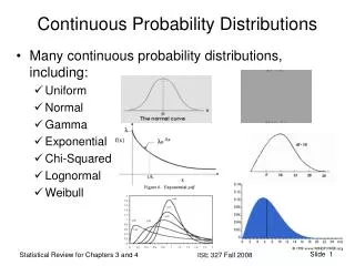
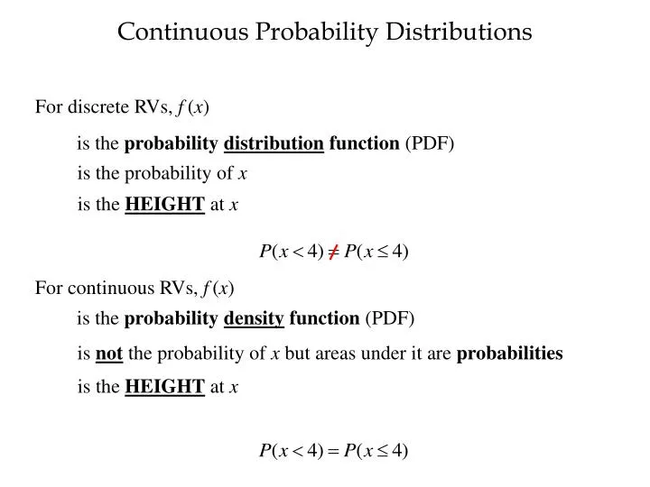
Continuous Probability Distributions. For discrete RVs, f ( x ). is the probability distribution function (PDF). is the probability of x. is the HEIGHT at x. For continuous RVs, f ( x ). is the probability density function (PDF).

E N D
Continuous Probability Distributions For discrete RVs, f(x) is the probability distribution function (PDF) is the probability of x is the HEIGHT at x For continuous RVs, f(x) is the probability density function (PDF) is not the probability of x but areas under it are probabilities is the HEIGHT at x
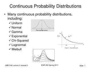
Continuous Probability Distributions The probability of the random variable assuming a value within some given interval from x1 to x2 is defined to be the area under the graph of the probability density function that is between x1and x2. P(x1 < x < x2) = area Uniform Normal Exponential x x x x2 x1 x2 x1 x1 x2
Uniform Probability Distribution Example: Slater's Buffet Slater customers are charged for the amount of salad they take. Sampling suggests that the amount of salad taken is uniformly distributed between 5 ounces and 15 ounces. x a b = 1/10 f (x) = 1/(b – a) = 1/(15 – 5) E(x) = (b + a)/2 = (15 + 5)/2 = 10 Var(x) = (b – a)2/12 = (15 – 5)2/12 = 8.33 s = 8.330.5 = 2.886
Uniform Probability Distribution Uniform Probability Distribution for Salad Plate Filling Weight f(x) 1/10 x 0 5 10 15 Salad Weight (oz.)
Uniform Probability Distribution What is the probability that a customer will take between 12 and 15 ounces of salad? P(12 <x< 15) = (h)(w) = (1/10)(3) = .3 f(x) 1/10 x 12 0 5 10 15 Salad Weight (oz.)
Uniform Probability Distribution What is the probability that a customer will equal 12 ounces of salad? P(x = 12) = (h)(w) = (1/10)(0) = 0 f(x) f(x) 1/10 x 12 0 5 10 15 Salad Weight (oz.)
Normal Probability Distribution The normal probability distribution is widely used in statistical inference, and has many business applications. x is a normal distributed with mean m and standard deviation s ≈ 3.14159… e ≈ 2.71828… s skew = ? x
Normal Probability Distribution The mean can be any numerical value: negative, zero, or positive. s = 2 m = 4 m = 6 m = 8
Normal Probability Distribution The standard deviation determines the width and height s = 2 s = 3 s = 4 m = 6 • data_bwt.xls
Standard Normal Probability Distribution z is a random variable having a normal distribution with a mean of 0 and a standard deviation of 1. s = 1 z m = 0
Standard Normal Probability Distribution • Use the standard normal distribution to verify the Empirical Rule: 68.26% of values of a normal random variable are within 1 standard deviations of its mean. 95.44% of values of a normal random variable are within 2 standard deviations of its mean. 99.74% of values of a normal random variable are within 3 standard deviations of its mean.
Standard Normal Probability Distribution • Compute the probability of being within 3 standard deviations • from the mean First compute P(z< -3) = ? s = 1 ? z -3.00 0
Standard Normal Probability Distribution P(z< -3.00) = ? column = .00 row = -3.0 P(z< -3) = .0013
Standard Normal Probability Distribution • Compute the probability of being within 3 standard deviations • from the mean s = 1 P(z< -3) = .0013 .0013 z -3.00 0
Standard Normal Probability Distribution • Compute the probability of being within 3 standard deviations • from the mean Next compute P(z> 3) = ? s = 1 ? z 3.00 0
Standard Normal Probability Distribution P(z< 3.00) = ? column = .00 row = 3.0 P(z< 3) = .9987
Standard Normal Probability Distribution • Compute the probability of being within 3 standard deviations • from the mean s = 1 P(z< 3) = .9987 P(z> 3) = 1 – .9987 .9987 .0013 z 3.00 0
Standard Normal Probability Distribution • Compute the probability of being within 3 standard deviations • from the mean s = 1 .9974 .0013 .0013 z 3.00 -3.00 0 99.74% of values of a normal random variable are within 3 standard deviations of its mean.
Standard Normal Probability Distribution • Compute the probability of being within 2 standard deviations • from the mean First compute P(z< -2) = ? s = 1 ? z -2.00 0
Standard Normal Probability Distribution P(z< -2.00) = ? column = .00 row = -2.0 P(z< -2) = .0228
Standard Normal Probability Distribution • Compute the probability of being within 2 standard deviations • from the mean s = 1 P(z< -2) = .0228 .0228 z -2.00 0
Standard Normal Probability Distribution • Compute the probability of being within 2 standard deviations • from the mean Next compute P(z> 2) = ? s = 1 ? z 2.00 0
Standard Normal Probability Distribution P(z< 2.00) = ? column = .00 row = 2.0 P(z< 2) = .9772
Standard Normal Probability Distribution • Compute the probability of being within 2 standard deviations • from the mean s = 1 P(z< 2) = .9772 P(z> 2) = 1 – .9772 .9772 .0228 z 2.00 0
Standard Normal Probability Distribution • Compute the probability of being within 2 standard deviations • from the mean s = 1 .9544 .0228 .0228 z -2.00 2.00 0 95.44% of values of a normal random variable are within 2 standard deviations of its mean.
Standard Normal Probability Distribution • Compute the probability of being within 1 standard deviations • from the mean First compute P(z< -1) = ? s = 1 ? z -1.00 0
Standard Normal Probability Distribution P(z< -1.00) = ? column = .00 row = -1.0 P(z< -1) = .1587
Standard Normal Probability Distribution • Compute the probability of being within 1 standard deviations • from the mean s = 1 P(z< -1) = .1587 .1587 z -1.00 0
Standard Normal Probability Distribution • Compute the probability of being within 1 standard deviations • from the mean Next compute P(z> 1) = ? s = 1 ? z 1.00 0
Standard Normal Probability Distribution P(z< 1.00) = ? column = .00 row = 1.0 P(z< 1) = .8413
Standard Normal Probability Distribution • Compute the probability of being within 1 standard deviations • from the mean s = 1 P(z< 1) = .8413 P(z> 1) = 1 – .8413 .8413 .1587 z 1.00 0
Standard Normal Probability Distribution • Compute the probability of being within 1 standard deviations • from the mean s = 1 .6826 .1587 .1587 z -1.00 1.00 0 68.26% of values of a normal random variable are within 1 standard deviations of its mean.
Standard Normal Probability Distribution Probabilities for the normal random variable are given by areas under the curve. Verify the following: The area to the left of the mean is .5 P(z< 0) = ? s = 1 ? z 0
Standard Normal Probability Distribution P(z< 0.00) = ? column = .00 row = 0.0 P(z< 0) = .5000
Standard Normal Probability Distribution Probabilities for the normal random variable are given by areas under the curve. Verify the following: The area to the left of the mean is .5 P(z< 0) = 0.5000 s = 1 .5000 z 0
Standard Normal Probability Distribution Probabilities for the normal random variable are given by areas under the curve. Verify the following: The area to the right of the mean is .5 P(z> 0) = 1 – .5000 s = 1 .5000 z 0
Standard Normal Probability Distribution Probabilities for the normal random variable are given by areas under the curve. Verify the following: The total area under the curve is 1 s = 1 1.0000 .5000 .5000 z 0
Standard Normal Probability Distribution • What is the probability that z is less than or equal to -2.76 s = 1 P(z< -2.76) = ? ? z -2.76 0
Standard Normal Probability Distribution P(z< -2.76) = ? column = .06 row = -2.7 P(z< -2.76) = .0029
Standard Normal Probability Distribution • What is the probability that z is less than or equal to -2.76? s = 1 P(z< -2.76) = .0029 .0029 z -2.76 0 P(z < -2.76) = .0029 • What is the probability that z is less than -2.76?
Standard Normal Probability Distribution • What is the probability that z is greater than or equal to -2.76? s = 1 P(z> -2.76) = 1 – .0029 = .9971 .9971 .0029 z -2.76 0 P(z > -2.76) = .9971 • What is the that z is greater than -2.76?
Standard Normal Probability Distribution • What is the probability that z is less than or equal to 2.87 P(z< 2.87) = ? s = 1 ? z 2.87 0
Standard Normal Probability Distribution P(z< 2.87) = ? column = .07 row = 2.8 P(z< 2.87) = .9979
Standard Normal Probability Distribution • What is the probability that z is less than or equal to 2.87 P(z< 2.87) = .9979 s = 1 .9979 z 2.87 0 P(z < 2.87) = .9971 • What is the probability that z is less than 2.87?
Standard Normal Probability Distribution • What is the probability that z is greater than or equal to 2.87? s = 1 P(z> 2.87) = 1 – .9979 = .0021 .9979 .0021 z 2.87 0 P(z > 2.87) = .0021 • What is the that z is greater than 2.87?
Standard Normal Probability Distribution • What is the value of z if the probability of being smaller than itis .0250? P(z<?) = .0250 s = 1 .0250 z ? 0
Standard Normal Probability Distribution • What is the value of z if the probability of being smaller than itis .0250? z = -1.96 column = .06 row = -1.9 P(z< -1.96) = .0250
Standard Normal Probability Distribution less • What is the value of z if the probability of being greater than itis .0192? .9808? P(z > ?) = .0192 s = 1 .9808 .0192 z ? 0
Standard Normal Probability Distribution less • What is the value of z if the probability of being greater than itis .0192? .9808? z = 2.07 column = .07 row = 2.0 P(z< 2.07) = .9808
Standard Normal Probability Distribution • What is the value of -z and z if the probability of being • between them is .9500? s = 1 If the area in the middle is .95 then the area NOT in the middle is .05 and so each tail has an area of .025 .9500 .0250 .0250 z -z z 0