Download
1 / 15
150 likes | 252 Views
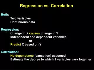
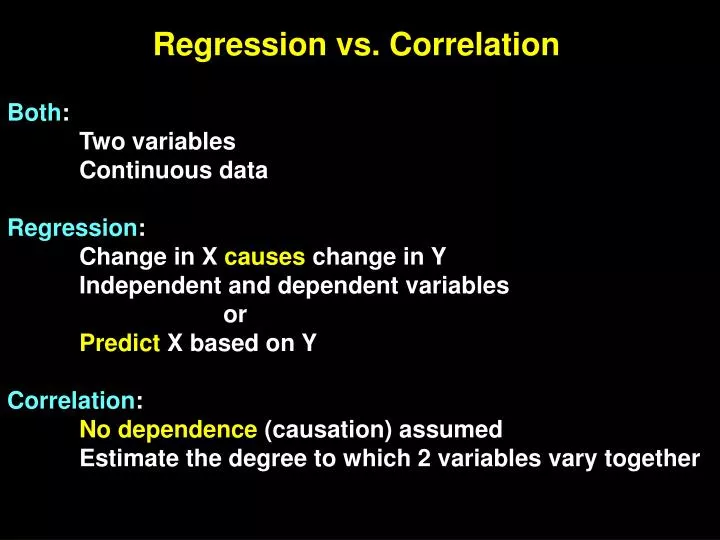
Regression vs. Correlation. Both : Two variables Continuous data Regression : Change in X causes change in Y Independent and dependent variables or Predict X based on Y Correlation : No dependence (causation) assumed Estimate the degree to which 2 variables vary together.

E N D
Regression vs. Correlation Both: Two variables Continuous data Regression: Change in X causes change in Y Independent and dependent variables or Predict X based on Y Correlation: No dependence (causation) assumed Estimate the degree to which 2 variables vary together
Correlation: more on bivariate statistics No dependence (causation) assumed Can call variables XY or X1X2 Are to variables independent, or do they covary
Visualize Correlation positive negative Y(X2) Y(X2) X1 X1 Increase in X associated with increase in Y Increase in X associated with decrease in Y
No correlation No correlation Y(X2) Y(X2) X1 X1 horizontal vertical
Pearson product-moment correlation coefficient Summed products of deviations of x & y xy = r = x2 y2 ss X * ss Y [(x-xbar) *(y-ybar)] = (x-xbar)2 * (y-ybar)2
Equivalent calculations (1) xy r = (n-1) sxsy Where sx = SD X sy = SD Y
Equivalent calculations (2) (Ŷi-Ybar)2 regression SS = = (r2) (Yi-Ybar)2 total SS regression SS r= r2 = total SS
Testing significance: H0: r () = 0 Assumes that data come from bivariate normal distribution true population parameter
r t = sr SE of r 1-r2 sr = n-2 Reject null if…… t calc > t(2),
data start; infile 'C:\Documents and Settings\cmayer3\My Documents\teaching\Biostatistics\Lectures\monitoring data for corr.csv' dlm=',' DSD; input year day site $ depth temp DO spCond turb pH Kpar secchi alk Chla; options ls=180; procprint; data one; set start; options ls=100; proccorr; var temp DO spCond turb pH Kpar secchi alk Chla; Correlations on raw data data two; set start; lnturb=log(turb); Create new variables by transformation lnsecchi=log(secchi); lgturb=log10(turb); lgsecchi=log10(secchi); sqturb=sqrt(turb); sqsecchi=sqrt(secchi); procprint; data three; set two; Correlations on transformed data proccorr; var lnturb lnsecchi; proccorr; var lgturb lgsecchi; proccorr; var sqturb sqsecchi; data four; set two; Plot raw and transformed options ls=100; procplot; plot turb*secchi; plot lnturb*lnsecchi; plot lgturb*lgsecchi; plot sqturb*sqsecchi; run;
Pearson Correlation Coefficients Prob > |r| under H0: Rho=0 Number of Observations temp DO spCond turb pH Kpar secchi alk Chla temp 1.00000 -0.21792 0.06538 -0.14523 0.35328 -0.23911 0.15689 0.11311 0.37612 0.0302 0.5202 0.1515 0.0003 0.1541 0.1209 0.3895 0.0001 99 99 99 99 99 37 99 60 99 DO -0.21792 1.00000 0.01542 -0.21550 0.50679 -0.24013 -0.06504 0.15790 0.38699 0.0302 0.8796 0.0322 <.0001 0.1523 0.5224 0.2282 <.0001 99 99 99 99 99 37 99 60 99 spCond 0.06538 0.01542 1.00000 0.48214 -0.29017 0.78394 -0.51332 0.74021 0.21367 0.5202 0.8796 <.0001 0.0036 <.0001 <.0001 <.0001 0.0337 99 99 99 99 99 37 99 60 99 turb -0.14523 -0.21550 0.48214 1.00000 -0.33727 0.89941 -0.50336 0.47441 0.07208 0.1515 0.0322 <.0001 0.0006 <.0001 <.0001 0.0001 0.4783 99 99 99 99 99 37 99 60 99 pH 0.35328 0.50679 -0.29017 -0.33727 1.00000 -0.56355 0.14049 -0.14061 0.61033 0.0003 <.0001 0.0036 0.0006 0.0003 0.1654 0.2839 <.0001 99 99 99 99 99 37 99 60 99 Kpar -0.23911 -0.24013 0.78394 0.89941 -0.56355 1.00000 -0.76680 0.85542 0.04579 0.1541 0.1523 <.0001 <.0001 0.0003 <.0001 <.0001 0.7878 37 37 37 37 37 37 37 29 37 secchi 0.15689 -0.06504 -0.51332 -0.50336 0.14049 -0.76680 1.00000 -0.49649 -0.30918 0.1209 0.5224 <.0001 <.0001 0.1654 <.0001 <.0001 0.0018 99 99 99 99 99 37 99 60 99 alk 0.11311 0.15790 0.74021 0.47441 -0.14061 0.85542 -0.49649 1.00000 0.12410 0.3895 0.2282 <.0001 0.0001 0.2839 <.0001 <.0001 0.3448 60 60 60 60 60 29 60 60 60 Chla 0.37612 0.38699 0.21367 0.07208 0.61033 0.04579 -0.30918 0.12410 1.00000 0.0001 <.0001 0.0337 0.4783 <.0001 0.7878 0.0018 0.3448 99 99 99 99 99 37 99 60 99
Nonparametric statistics Sometimes called distribution free statistics because they do not require that the data fit a normal distribution Many nonparametric procedures are based on ranked data. Data are ranked by ordering them from lowest to highest and assigning them, in order, the integer values from 1 to the sample size.
Data transformations Data transformation can “correct” deviation from normality and uneven variance (heteroscedasticity) See chapter 13 in Zar Pretty much….. Whatever works, works. Some common ones are for % or proportion use asin of square root log10 for density (#/m2) Right transformation can allow you to use parametric statistics