Download
1 / 40
440 likes | 760 Views
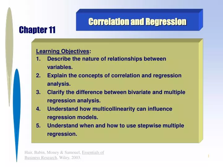
Chapter 11. Correlation and Regression. Learning Objectives : Describe the nature of relationships between variables. Explain the concepts of correlation and regression analysis. Clarify the difference between bivariate and multiple regression analysis.

E N D
Chapter 11 Correlation and Regression Learning Objectives: • Describe the nature of relationships between variables. • Explain the concepts of correlation and regression analysis. • Clarify the difference between bivariate and multiple regression analysis. • Understand how multicollinearity can influence regression models. • Understand when and how to use stepwise multiple regression.
Concepts About Relationships Presence Nature Direction Go On-Line www.technology.com Strength of Association
Relationship Presence ? . . . . assesses whether a systematic relationship exists between two or more variables. If we find statistical significance between the variables we say a relationship is present.
Nature of Relationships Relationships between variables typically are described as either linear or nonlinear. Linear relationship = a “straight-line association” between two or more variables. Nonlinear relationship = often referred to as curvilinear, it is best described by a curve instead of a straight line.
Direction of Relationship The direction of a relationship can be either positive or negative. • Positive relationship = when one variable increases, e.g., loyalty to employer, then so does another related one, e.g. effort put forth for employer. • Negative relationship = when one variable increases, e.g., satisfaction with job, then a related one decreases, e.g. likelihood of searching for another job.
Strength of Association When a consistent and systematic relationship is present, the researcher must determine the strength of association. The strength ranges from very strong to slight.
Covariation . . . . exists when one variable consistently and systematically changes relative to another variable. The correlation coefficient is used to assess this linkage.
Correlation Coefficients: What do they mean? + 1.0 0.0 Zero Correlation = the value of Y does not increase or decrease with the value of X. - 1.0 Positive Correlation = when the value of X increases, the value of Y also increases. When the value of X decreases, the value of Y also decreases. Negative Correlation = when the value of X increases, the value of Y decreases. When the value of X decreases, the value of Y increases.
Exhibit 11-1 Rules of Thumb about Correlation Coefficient Size Coefficient Strength of Range Association +/– .91 to +/– 1.00 Very Strong +/– .71 to +/– .90 High +/– .41 to +/– .70 Moderate +/– .21 to +/– .40 Small +/– .01 to +/– .20 Slight
Pearson Correlation The Pearson correlation coefficient measures the linear association between two metric variables. It ranges from – 1.00 to + 1.00, with zero representing absolutely no association. The larger the coefficient the stronger the linkage and the smaller the coefficient the weaker the relationship.
Coefficient of Determination The coefficient of determination is the square of the correlation coefficient, or r2. It ranges from 0.00 to 1.00 and is the amount of variation in one variable explained by one or more other variables.
Exhibit 11-3 Bivariate Correlation Between Work Group Cooperation and Intention to Search for another Job Descriptive Statistics
Exhibit 11-3 Bivariate Correlation Between Work Group Cooperation and Intention to Search for another Job Correlations * Coefficient is significant at the 0.01 level (2-tailed).
Exhibit 11-5 Bar Charts for Rankings for Food Quality and Atmosphere
Exhibit 11-4 Correlation of Food Quality and Atmosphere Using Spearman’s rho * Coefficient is significant at the 0.01 level (2-tailed).
Exhibit 11-6 Customer Rankings of Restaurant Selection Factors Statistics
Exhibit 11-8 Definitions of Statistical Techniques ANOVA (analysis of variance) is used to examine statistical differences between the means of two or more groups. The dependent variable is metric and the independent variable(s) is nonmetric. One-way ANOVA has a single nonmetric independent variable and two-way ANOVA can have two or more nonmetric independent variables. Bivariate regression has a single metric dependent variable and a single metric independent variable. Cluster analysis enables researchers to place objects (e.g., customers, brands, products) into groups so that objects within the groups are similar to each other. At the same time, objects in any particular group are different from objects in all other groups. Correlation examines the association between two metric variables. The strength of the association is measured by the correlation coefficient. Conjoint analysis enables researchers to determine the preferences individuals have for various products and services, and which product features are valued the most.
Exhibit 11-8 Definitions of Statistical Techniques Discriminant analysis enables the researcher to predict group membership using two or more metric dependent variables. The group membership variable is a nonmetric dependent variable. Factor analysis is used to summarize the information from a large number of variables into a much smaller number of variables or factors. This technique is used to combine variables whereas cluster analysis is used to identify groups with similar characteristics. Logistic regression is a special type of regression that can have a non-metric/categorical dependent variable. Multiple regression has a single metric dependent variable and several metric independent variables. MANOVA is similar to ANOVA, but it can examine group differences across two or more metric dependent variables at the same time. Perceptual mapping uses information from other statistical techniques to map customer perceptions of products, brands, companies, and so forth.
Exhibit 11-10 Bivariate Regression of Satisfaction and Food Quality Descriptive Statistics
Exhibit 11-10 Bivariate Regression of Satisfaction and Food Quality Model Summary *Predictors: (Constant), X1 – Excellent Food Quality
Exhibit 11-11 Other Aspects of Bivariate Regression *Predictors: (Constant), X1 – Excellent Food Quality Dependent Variable: X17 – Satisfaction
Exhibit 11-11 Other Aspects of Bivariate Regression continued Coefficients *Dependent Variable: X17 – Satisfaction
Calculating the “Explained” and “Unexplained” Variance in Regression The explained variance in regression, referred to as r2, is calculated by dividing the regression sum of squares by the total sum of squares. For example, in Exhibit 11-11, divide the regression sum of squares for Samouel’s of 35.00l by 133.160 and you get .263. The unexplained variance in regression, referred to as residual variance, is calculated by dividing the residual sum of squares by the total sum of squares. For example, in Exhibit 11-11, divide the residual sum of squares for Samouel’s of 98.159 by 133.160 and you get .737. This tells us that a lot of variance (73.7%) in the dependent variable in not explained by this regression equation.
How to calculate the t-value? The t-value is calculated by dividing the regression coefficient by its standard error. In Exhibit 11-11 in the Coefficients table, if you divide the Unstandardized Coefficient for Samouel’s of .459 by the Standard Error of .078, the result will be a t-value of 5.8846. Note that the number in the table for the t-value is 5.911. The difference between the calculated 5.8846 and the 5.911 reported in the table is due to the fact that the computer reported the “rounded off” numbers for the Unstandardized Coefficient and the Standard Error but the t-value is calculated and reported without rounding.
How to interpret the regression coefficient ? The regression coefficient of .459 for Samouel’s X1– Food Quality reported in Exhibit 11-11 is interpreted as follows: “ . . . for every unit that X1 increases, X17 will increase by .459 units.” Recall that in this example X1 is the independent (predictor) variable and X17 is the dependent variable.
Exhibit 11-13 Multiple Regression of Return in Future and Food Independent Variables Descriptive Statistics
Exhibit 11-13 Multiple Regression of Return in Future and Food Independent Variables (continued) Model Summary *Predictors: (Constant), X9 – Wide Variety of Menu Items, X1 – Excellent Food Quality, X4 – Excellent Food Taste Dependent Variable: X18 – Return in Future
Exhibit 11-14 Other Information for Multiple Regression Models ANOVA *Predictors: (Constant), X9 – Wide Variety of Menu Items, X1 – Excellent Food Quality, X4 – Excellent Food Taste Dependent Variable: X18 – Return in Future
Exhibit 11-14 Other Information for Multiple Regression Models Coefficients* *Dependent Variable: X18 – Return in Future
Exhibit 11-17 Summary Statistics for Employee Regression Model Model Summary *Predictors: (Constant), X12 – Benefits Reasonable, X9 – Pay Reflects Effort, X1 – Paid Fairly Dependent Variable: X14 – Effort
Exhibit 11-18 Coefficients for Employee Regression Model Coefficients* *Dependent Variable: X14 – Effort
Exhibit 11-19 Bivariate Correlations of Effort and Compensation Variables Pearson Correlations
Exhibit 11-19 Bivariate Correlations of Effort and Compensation Variables Statistical Significance of Pearson Correlations (1 – tailed)
Exhibit 11-20 Stepwise Regression Based on Samouel’s Customer Survey Model Summary *Predictors: (Constant), X1 – Excellent Food Quality, X6 – Friendly Employees Dependent Variable: X17 – Satisfaction
Exhibit 11-20 Stepwise Regression Based on Samouel’s Customer Survey ANOVA *Predictors: (Constant), X1 – Excellent Food Quality, X6 – Friendly Employees Dependent Variable: X17 – Satisfaction
Exhibit 11-21 Means and Correlations for Selected Variables from Samouel’s Customer Survey Descriptive Statistics
Exhibit 11-20 Independent Variables in Stepwise Regression Model ANOVA *Predictors: (Constant), X1 – Excellent Food Quality, X6 – Friendly Employees Dependent Variable: X17 – Satisfaction
Exhibit 11-23 Coefficients for Stepwise Regression Model Coefficients* *Dependent Variable: X17 – Satisfaction
Correlation and Regression Go On-Line www.yankelovich.com How can business researchers use the data from the research reported on this website?